The Rasch Paradigm: Revolution or Normal Progression?

Much of the historical and philosophical analysis (e.g., Engelhard, Fisher) from the Rasch camp has followed the notion that Rasch’s principles and methods flow naturally and logically from the best measurement thinking (Thurstone, Binet, Guttman, Terman, et al.) of the early 20th century and beyond. From this very respectable and defensible perspective, Rasch’s contribution was a profound, but normal progression based on this earlier work and provided the tools to deal with the awkward measurement problems of the time, e.g. validity, reliability, equating. Before Rasch, the consensus was the only forms that could be equated were those that didn’t need equating.

When I reread Thomas Kuhn’s “The Structure of Scientific Revolutions” I was led to the conclusion that Rasch’s contribution rises to the level of a revolution, not just a refinement of earlier thinking or elaboration of previous work. It is truly a paradigm shift, although Kuhn didn’t particularly like the phrase (and it probably doesn’t appear in my 1969 edition of “Structure”.) I don’t particularly like it because it doesn’t adequately differentiate between “new paradigm” and “tweaked paradigm”; in more of Kuhn’s words, a new world, not just a new view of an old world.

To qualify as a Kuhnian Revolution requires several things: the new paradigm, of course, which needs to satisfactorily resolve the anomalies that have accumulated under the old paradigm, which were sufficient to provoke a crisis in the field. It must be appealing enough to attract a community of adherents. To attract adherents, it must solve enough of the existing puzzles to be satisfying and it must present some new ones to send the adherents in a new direction and give them something new to work on.

One of Kuhn’s important contributions was his description of “Normal Science,” which is what most scientists do most of the time. It can be the process of eliminating inconsistencies, either by tinkering with the theory or by disqualifying observations. It can be clarifying details or bringing more precision to the experimentation. It can be articulating implications of the theory, i.e., if that is, then this must be. We get more experiments to do and other hypotheses to proof.

Kuhn described this process as “Puzzle Solving,” with, I believe, no intent of being dismissive. These fall into the rough categories of tweaking the theory, designing better experiments, or building better instruments.

The term “paradigm” wasn’t coined by Kuhn but he certainly brought it to the fore. There has been a lot of discussion and criticism since of the varied and often casual ways he used the word but it seems to mean the accepted framework within which the community who accept the framework perform normal science. I don’t think that is as circular as it seems.

The paradigm defines the community and the community works on the puzzles that are “normal science” under the paradigm. The paradigm can be ‘local’ existing as an example or, perhaps even an exemplar of the framework. Or it can be ‘global.’ Then it is the view that defines a community of researchers and the world view that holds that community together. This requires that it be attractive enough to divert adherents from competing paradigms and that it be open-ended enough to give them issues to work on or puzzles to solve.

If it’s not attractive, it won’t have adherents. The attraction has to be more than just able to “explain” the data more precisely. Then it would just be normal science with a better ruler. To truly be a new paradigm, it needs to involve a new view of the old problems. One might say, and some have, that after, say, Aristotle and Copernicus and Galileo and Newton and Einstein and Bohr and Darwin and Freud, etc., etc., we were in a new world.

Your paradigm won’t sell or attract adherents if it doesn’t give them things to research and publish. The requirement that the paradigm be open-ended is more than marketing. If it’s not open-ended, then it has all the answers, which makes it dogma or religion, not science.

Everything is fine until it isn’t. Eventually, an anomaly will present itself that can’t be explained away by tweaking the theory, censoring the data, or building a better microscope. Or perhaps, anomalies and the tweaks required to fit them in become so cumbersome, the whole thing collapses of its own weight.  When the anomalies become too obvious to dismiss, too significant to ignore, or too cumbersome to stand, the existing paradigm cracks, ‘normal science’ doesn’t help, and we are in a ‘crisis’.

Crisis

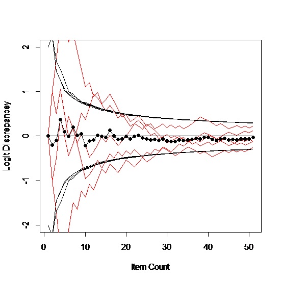
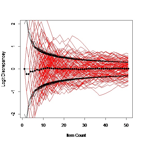
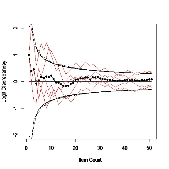
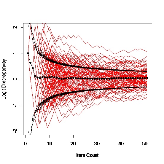
The psychometric new world may have turned with Lord’s seminal 1950 thesis. (Like most of us at a similar stage, Lord’s crisis was he needed a topic that would get him admitted into the community of scholars.) When he looked at a plot of item percent correct against total number correct (the item’s characteristic curve), he saw a normal ogive. That fit his plotted data pretty well, except in the tails. So he tweaked the lower end to “explain” too many right answers from low scorers. The mathematics of the normal ogive are, at least, cumbersome and, in 1950, computationally intractable. So that was pretty much that, for a while.

In the 1960s, the normal ogive morphed into the logistic, perhaps the idea came from following Rasch’s (1960) lead, perhaps from somewhere else, perhaps due to Birnbaum (1968); I’m not a historian and this isn’t a history lesson. The mathematics were a lot easier and computers were catching up. The logistic was winning out but with occasional retreats to the the normal ogive because it fit a little better in the tails .

US psychometricians saw the problem as data fitting and it wasn’t easy. There were often too many parameters to estimate without some clever footwork. But we’re clever and most of those computational obstacles have been overcome to the satisfaction of most. The nagging questions remaining are more epistemological than computational.

Can we know if our item discrimination estimates are truly indicators of item "quality" and not loadings on some unknown, extraneous factor(s)?

If the lower asymptote is what happens at minus infinity where we have no data and never want to have any, why do we even care?

If the lower asymptote is the probability of a correct response from an examinee with infinitely low ability, how can it be anything but 1/k, where k is the number of response choices?

How can the lower asymptote ever be higher than 1/k? (See Slumdog Millionaire, 2008)

If the lower asymptote is population-dependent, isn't the ability estimate dependent on the population we choose to assign the person to? Mightn't individuals vary in their propensity to respond to items they don't know.

Wouldn't any population-dependent estimate be wrong on the level of the individual?

If you ask the data for “information” beyond the sufficient statistics, not only are your estimates population-dependent, they are subject to whatever extraneous factors that might separate high scores from low scores in that population. This means sacrificing validity in the name of reliability.

Rasch did not see his problem as data fitting. As an educator, he saw it directly: more able students do better on the set tasks than less able students. As an associate of Ronald Fisher (either the foremost statistician of the twentieth century who also made contributions to genetics or the foremost geneticist of the twentieth century who also made contributions to statistics), Rasch knew about logistic growth models and sufficient statistics. Anything left in the data, after reaping the information with the sufficient statistics, should be noise and should be used to control the model. The size of the residuals isn’t as interesting as the structure, or lack thereof.¹

Rasch Measurement Theory certainly has its community and the members certainly adhere and seem to find enough to do. Initially, Rasch found his results satisfying because it got him around the vexing problem of how to assess the effectiveness of remedial reading instruction when he didn’t have a common set of items or common set of examinees over time. This led him to identify a class of models that define Specific Objectivity.

Rasch’s crisis (how to salvage a poorly thought-out experiment) hardly rises to the epic level of Galileo’s crisis with Aristotle, or Copernicus’ crisis with Ptolemy, or Einstein’s crisis with Newton. A larger view would say the crisis came about because the existing paradigms did not lead us to “measurement”, as most of science would define it.

In the words of William Thomson, Lord Kelvin:

When you can measure what you are speaking about and express it in numbers, you know something about it; but when you cannot measure it, when you cannot express it in numbers, your knowledge is of a meager and unsatisfactory kind.

Revolution

Rasch’s solution did change the world for any adherents who were willing to accept his principles and follow his methods. They now knew how to ‘equate’ scores from disparate instruments, but beyond that, how to develop scales for measuring, define constructs to be measured, and do better science.

Rasch’s solution to his problem in the 1950s with remedial reading scores is still the exemplar and “local” definition of the paradigm. His generalization of that solution to an entire class of models and his exposition of “specific objectivity” are the “global” definition. (Rasch, 1960) 

There’s a problem with all this. I am trying to force fit Rasch’s contribution into Kuhn’s “Structure of Scientific Revolutions” paradigm when Rasch Measurement admittedly isn’t science. It’s mathematics, or statistics, or psychometrics; a tool, certainly a very useful tool, like Analysis of Variance or Large Hadron Colliders.

Measures are necessary precursors to science. Some of the weaknesses in pre-Rasch thinking about measurement are suggested in the following koans, hoping for enlightened measurement, not Zen enlightenment.

"Whatever exists at all exists in some amount. To know it thoroughly involves knowing its quantity as well as its quality." E. L. Thorndike

"Within the range of objects for which the measuring instrument is intended, its function must be independent of the object of measurement." L. L. Thurstone

"You never know a line is crooked unless you have a straight one to put next to it." Socrates

"Correlations are population-dependent, and therefore scientifically rather uninteresting." Georg Rasch

"We can act as though measured differences along the latent trait are distances on a river but whoever is piloting better watch for meanders and submerged rocks."

"We may be trying to measure size; perhaps height and weight would be better. Or perhaps, we are measuring 'weight', when we should go after 'mass'"

"The larger our island of knowledge, the longer our shoreline of wonder." Ralph W. Sockman

"The most exciting thing to hear in science ... is not 'Eureka' but 'That's funny.'" Isaac Asimov

1A subtitle for my own dissertation could be “Rasch’s errors are my data.”

The Five ‘S’s to Rasch Measurement

The mathematical, statistical, and philosophical faces of Rasch measurement are separability, sufficiency, and specific objectivity. ‘Separable’ because the person parameter and the item parameter interact in a simple way; Β/Δ in the exponential metric or β-δ in the log metric. ‘Sufficient’ because ‘nuisance’ parameters can be conditioned out so that, in most cases, the number of correct responses is the sufficient statistic for the person’s ability or the item’s difficulty. Specific Objectivity is Rasch’s term for ‘fundamental measurement’; what Wright called ‘sample-free item calibration’. It is objective because it does not depend on the specific sample of items or people; it is specific because it may not apply universally and the validity in any new application must be established.

I add two more ‘S‘s to the trinity: simplicity and symmetry.

Simplicity

We have talked ad nauseum about simplicity. It in fact is one of my favorite themes. The chances that the person will answer the item correctly is Β / (Β + Δ), which is about as simple as life gets.1 Or in less-than-elegant prose:

The likelihood that the person wins is the odds of the person winning
divided by sum of the odds for person winning and the odds for the item winning.

With such a simple model, the sufficient statistics are simple counts, and the estimators can be as simple as row averages. Rasch (1960) did many of his analyses graphically; Wright and Stone (1979) give algorithms for doing the arithmetic, somewhat laboriously, without the benefit of a computer. The first Rasch software at the University of Chicago (CALFIT and BICAL) ran on a ‘mini-computer’ that wouldn’t fit in your kitchen and had one millionth the capacity of your phone.

Symmetry

The first level of symmetry with Rasch models is that person ability and item difficulty have identical status. We can flip the roles of ability and difficulty in everything I have said in this post and every preceding one, or in everything Rasch or Gerhardt Fischer has ever written, and nothing changes. It makes just as much sense to say Δ / (Δ + Β) as Β / (Β + Δ). Granted we could be talking about anti-ability and anti-difficulty, but all the relationships are just the same as before. That’s almost too easy.

Just as trivially, we have noted, or at least implied, that we can flip, as suits our purposes, between the logistic and exponential expressions of the models without changing anything. In the exponential form, we are dealing with the odds that a person passes the standard item; in the logistic form, we have the log odds. If we observe one, we observe the other and the relationships among items and students are unchanged in any fundamental way. We are not limited to those two forms. Using base e is mathematically convenient, but we can choose any other base we like; 10, or 100, or 91 are often used in converting to ‘scale scores’. Any of these transformations preserves all the relationships because they all preserve the underlying interval scale and the relative positions of objects and agents on it.

That’s the trivial part.

Symmetry was a straightforward concept in mathematics: Homo sapiens, all vertebrates, and most other fauna have bilateral symmetry; a snowflake has sixfold; a sphere an infinite number. The more degrees of symmetry, the fewer parameters that are required to describe the object. For a sphere, only one, the radius, is needed and that’s as low as it goes.

Leave it to physicists to take an intuitive idea and made it into a topic for advanced graduate seminars2:

A symmetry of a physical system is a physical or mathematical feature of the system
(observed or intrinsic)
that is preserved or remains unchanged under some transformation. 

For every invariant (i.e., symmetry) in the universe, there is a conservation law.
Equally, for every conservation law in physics, there is an invariant.
(Noether’s Theorem, 1918)3.

Right. I don’t understand enough of that to wander any deeper into space, time, or electromagnetism or to even know if this sentence makes any sense.

In Rasch’s world,4 when specific objectivity holds, the ‘difficulty’ of an item is preserved whether we are talking about high ability students or low, fifth graders or sixth, males or females, North America or British Isles, Mexico or Puerto Rico, or any other selection of students that might be thrust upon us.

Rasch is not suggesting that the proportion answering the item correctly (aka, p-value) never varies or that it doesn’t depend on the population tested. In fact, just the opposite, which is what makes p-values and the like ” rather scientifically uninteresting”. Nor do we suggest that the likelihood that a third grader will correctly add two unlike fractions is the same as the likelihood for a nineth grader. What we are saying is that there is an aspect of the item that is preserved across any partitioning of the universe; that the fraction addition problem has its own intrinsic difficulty unrelated to any student.

“Preserved across any partitioning of the universe” is a very strong statement. We’re pretty sure that kindergarten students and graduate students in Astrophysics aren’t equally appropriate for calibrating a set of math items. And frankly, we don’t much care. We start caring if we observe different difficulty estimates from fourth-grade boys or girls, or from Blacks, Whites, Asians, or Hispanics, or from different ability clusters, or in 2021 and 2022. The task is to establish not if it ever fails but when symmetry holds.

I need to distinguish a little more carefully between the “latent trait” and our quantification of locations on the scale. An item has an inherent difficulty that puts it somewhere along the latent trait. That location is a property of the item and does not depend on any group of people that have been given, or that may ever be given the item. Nor does it matter if we choose to label it in yards or meters, Fahrenheit or Celsius, Wits or GRits. This property is what it is whether we use the item for a preschooler, junior high student, astrophysicist, or Supreme Court Justice. This we assume is invariant. Even IRTists understand this.

Although the latent trait may run the gamut, few items are appropriate for use in more than one of the groups I just listed. That would be like suggesting we can use the same thermometer to assess the status of a feverish preschooler that we use for the surface of the sun, although here we are pretty sure we are talking about the same latent ‘trait’. It is equally important to choose an appropriate sample for calibrating the items. A group of preschoolers could tell us very little about the difficulty of items appropriate for assessing math proficiency of astrophysicists.

Symmetry can break in our data for a couple reasons. Perhaps there is no latent trait that extends all the way from recognizing basic shapes to constructing proofs with vector calculus. I am inclined to believe there is in this case, but that is theory and not my call. Or perhaps we did not appropriately match the objects and agents. Our estimates of locations on the trait should be invariant regardless of which objects and agents we are looking at. If there is an issue, we will want to know why: are difficulty and ability poorly matched? Is there a smart way to get the item wrong? Is there a not-smart way to get it right? Is the item defective? Is the person misbehaving? Or did the trait shift? Is there a singularity?

My physics is even weaker that my mathematics.

What most people call ‘Goodness of Fit’ and Rasch called ‘Control of the Model’, we are calling an exploration of the limits of symmetry. For me, I have a new buzz word, but the question remains, “Why do bright people sometimes miss easy items and non-bright people sometimes pass hard items?”5 This isn’t astrophysics.

Here is my “item response theory”:

The Rasch Model is a main effects model; the sufficient statistics for ability and difficulty are the row and column totals of the item response matrix. Before we say anything important about the students or items, we need to verify that there are no interactions. This means no matter how we sort and block the rows, estimates of the column parameters are invariant (enough).

That’s me regressing to my classical statistical training to say that symmetry holds for these data.


[1] It may look more familiar but less simple if we rewrite it as (Β/Δ) / (1 + Β/Δ), even better eβ-δ/(1 + eβ-δ), but it’s all the same for any observer.

[2] Both of the following statements were lifted (plagiarized?) from a Wikipedia discussion of symmetry. I deserve no credit for the phrasing, nor do I seek it.

[3] Emmy Noether was a German mathematician whose contributions, among other things, changed the science of physics by relating symmetry and conservation. The first implication of her theorem was it solved Hilbert and Einstein’s problem that General Relativity appeared to violate the conservation of energy. She was generally unpaid and dismissed, notably and empathically not by Hilbert and Einstein, because she was a woman and a Jew. In that order.

When Göttingen University declined to give her a paid position, Hilbert responded, “Are we running a University or a bathing society?” In 1933, all Jews were forced out of academia in Germany; she spent the remainder of her career teaching young women at Bryn Mawr College and researching at the Institute for Advanced Study in Princeton (See Einstein, A.)

[4] We could flip this entire conversation and talk about the ‘ability’ of a person preserved across shifts of item difficulty, type, content, yada, yada, yada, and it would be equally true. But I repeat myself again.

[5] Except for the ‘boy meets girl, . . . aspect, this question is the basic plot of “Slumdog Millionaire“, undoubtedly the greatest psychometric movie ever made. I wouldn’t however describe the protagonist as “non-bright”, which suggests there is something innate in whatever trait is operating and exposes some of the flaws in my use of the rather pejorative term. I should use something more along the lines of “poorly schooled” or “untrained”, placing effort above talent.

Latent Trait Analysis or Item Response ‘Theory’?

In the 1960s, we had Latent Trait Analysis (Birnbaum, A., in Lord & Novack, 1968); in the 1970s, Darrell Bock lobbied for a new label ‘Item Response Theory’ (IRT) as more descriptive of what was actually going on. He was right about conventional psychometric practice in the US; he was wrong for condoning it as the reasonable thing to do. I am uncertain in what sense he used the word ‘theory’. We don’t seem to be talking about “a well-confirmed explanation of nature, in a way consistent with scientific method, and fulfilling the criteria required by modern science.” Maybe a theory of measurement would be better than a theory of item responses.

The ‘item response matrix’ is a means to an end. It is nothing more or less than rows and columns of ones and zeros recording which students answered which items correctly and which incorrectly.[1] It is certainly useful in the classroom for grading students and culling items; however, it is population dependent, and therefore scientifically rather uninteresting, like correlations and factor analysis. My interest in it is to harvest whatever the matrix can tell me about some underlying aspect of students.

The focus of IRT is estimate parameters to “best explain” the ones and zeros. “Explain” is used here in the rather sterile statistical sense of ‘minimize the residual errors’, which has long been a respectable activity in statistical practice. Once IRTists are done with their model estimation, the ‘tests of fit’ are typically likelihood ratio tests, which are relevant to the question, “Have we included enough parameters and built a big enough model?” and less relevant to “Why didn’t that item work?” or “Why did these students miss those items?”

Latent Trait Analysis’ is a more descriptive term for the harvesting of relevant information when our focus is on the aspect of the student that caused us to start this entire venture. Once all the information is extracted from the data, we will have located the students on an interval scale for a well-defined trait (the grading part). Anything left over is useful and essential for ‘controlling the model’, i.e., selecting, revising, or culling items and diagnosing students. Parameter estimation is only the first step toward understanding what happened: “explaining!” in the sense of ‘illuminating the underlying mechanism’.

“Grist” is grain separated from the chaff. The ones and zeros are grist for the measurement mill but several steps from sliced bread. The item response matrix is data carefully elicited from appropriate students using appropriate items to expose, isolate, and abstract the specific trait we are after. In addition to the chaff of extraneous factors, we need to deal with the nuisance parameters and insect parts as well.

Wright’s oft misunderstood phrases “person-free item calibration” and “item-free person measurement” (Wright, B. D., 1968) notwithstanding, it is still necessary to subject students to items before we make any inferences about the underlying trait. The problem is to make inferences that are “sample-freed”. The key, sine que non, and Rasch’s contribution that makes this possible was a class of models that had separable parameters leading to sufficient statistics ending at Specific Objectivity.

Describing Rasch latent trait models as a special case of 3PL IRT is Algebra 101 but fails to recognize the power and significance of sufficient statistics and the generality of his theory of measurement. Rasch’s Specific Objectivity is the culmination of the quest for Thurstone’s holy grail of ‘fundamental measurement’.


[1] For the moment, we will stick with the dichotomous case and talk in terms of educational assessment because it’s what I know, although it doesn’t change the argument to think polytomous responses in non-educational applications.

Lexiles: the making of a measure

PDF download: Using Lexiles Safely

A recent conversation with a former colleague (it was more of a one-way lecture) about what psychometricians don’t understand about students and education led me to resurrect an article that I wrote for the Rasch Measurement Transactions four or five years ago. It deals specifically with Lexiles© but it is really about how one defines and uses measures in education and science.

The antagonism toward Lexiles in particular and Rasch measures in general is an opportunity to highlight some distinctions between measurement and analysis and between a measure and an assessment. Often when trying to discuss the development of reading proficiency, specialists in measurement and reading seem to be talking at cross-purposes. Reverting to argument by metaphor, measurement specialists are talking about measuring weight; and reading specialists, about providing proper nutrition.

There is a great deal involved in physical development that is not captured when we measure a child’s weight and the process of measuring weight tells us nothing about whether the result is good, bad, or normal; if you should continue on as you are, schedule a doctor’s appointment, or go to the emergency room without changing your underwear. Evaluation of the result is an analysis that comes after the measurement and depends on the result being a measure. No one would suggest that, because it doesn’t define health, weight is not worth measuring or that it is too politically sensitive to talk about in front of nutritionists. A high number does not imply good nutrition nor does a low number imply poor nutrition. Nonetheless, the measurement of weight is always a part of an assessment of well-being.

A Lexile score, applied to a person, is a measure of reading ability[i], which I use to mean the capability to decode words, sentences, paragraphs, and Supreme Court decisions. Lexiles, as applied to a text, is a measure of how difficult the text is to decode. Hemingway’s “For Whom the Bell Tolls” (840 Lexile score) has been cited as an instance where Lexiles do not work. Because a 50th percentile sixth-grade reader could engage with this text, something must be wrong because the book was written for adults. This counter-example, if true, is an interesting case. I have two counter-counter-arguments: first, all measuring instruments have limitations to their use and, second, Lexiles may be describing Hemingway appropriately.

First, outside the context of Lexiles, there is always difficulty for either humans or computer algorithms in scoring exceptional, highly creative writing. (I would venture to guess that many publishers, who make their livings recognizing good writing[ii], would reject Hemingway, Joyce, or Faulkner-like manuscripts if they received them from unknown authors.) I don’t think it follows that we should avoid trying to evaluate exceptional writing. But we do need to know the limits of our instruments.

I rely, on a daily basis, on a bathroom scale. I rely on it even though I believe I shouldn’t use it on the moon, under water, or for elephants or measuring height. It does not undermine the validity of Lexiles in general to discover an extraordinary case for which it does not apply. We need to know the limits of our instrument; when does it produce valid measures and when does it not.

Second, given that we have defined the Lexile for a text as the difficulty of decoding the words and sentences, the Lexile analyzer may be doing exactly what it should with a Hemingway text. Decoding the words and sentences in Hemingway is not that hard: the vocabulary is simple, the sentences short. That’s pretty much what the Lexile score reflects.

Understanding or appreciating Hemingway is something else again. This may be getting into the distinction between reading ability, as I defined it, and reading comprehension, as the specialists define that. You must be able to read (i.e., decode) before you can comprehend. Analogously, you have to be able to do arithmetic before you can solve math word problems[iii]. The latter requires the former; the former does not guarantee the latter. Necessary but not sufficient.

The Lexile metric is a developmental scale that is not related to instructional method or materials, or to grade-level content standards. The metric reflects increasing ability to read, in the narrow sense of decode, increasingly advanced text. As students advance through the reading/language arts curriculum, they should progress up the Lexile scale. Effective, including standards-based, instruction in ELA[iv] should cause them to progress on the Lexile scale; analogously good nutrition should cause children to progress on the weight scale[v].

One could coach children to progress on the weight scale in ways counter to good nutrition[vi]. One might subvert Lexile measurements by coaching students to write with big words and long sentences. This does not invalidate either weight or reading ability as useful things to measure. There do need to be checks to ensure we are effecting what we set out to effect.

The role of standards-based assessment is to identify which constituents of reading ability and reading comprehension are present and which absent. Understanding imagery and literary devices, locating topic sentences, identifying main ideas, recognizing sarcasm or satire, comparing authors’ purposes in two passages are within its purview but are not considered in the Lexile score. Its analyzer relies on rather simple surrogates for semantic and syntactic complexity.

The role of measurement on the Lexile scale is to provide a narrowly defined measure of the student’s status on an interval scale that extends over a broad range of reading from Dick and Jane to Scalia and Sotomayor. The Lexile scale does not define reading, recognize the breadth of the ELA curriculum, or replace grade-level content standards-based assessment, but it can help us design instruction and target assessment to be appropriate to the student. We do not expect students to say anything intelligent about text they cannot decode, nor should we attempt to assess their analytic skills using such text.

Jack Stenner (aka, Dr. Lexile) uses as one of his parables, you don’t buy shoes for a child based on grade level but we don’t think twice about assigning textbooks with the formula (age – 5). It’s not one-size-fits-all in physical development. Cognitive development is probably no simpler if we were able to measure all its components. To paraphrase Ben Wright, how we measure weight has nothing to do with how skillful you are at football, but you better have some measures before you attempt the analysis.

[i] Ability may not be the best choice of a word. As used in psychometrics, ability is a generic placeholder for whatever we are trying to measure about a person. It implies nothing about where it came from, what it is good for, or how much is enough. In this case, we are using reading ability to refer to a very specific skill that must be taught, learned, and practiced.

[ii] It may be more realistic to say they make their livings recognizing marketable writing, but my cynicism may be showing.

[iii] You also have to decode the word problem but that’s not the point of this sentence. We assume, often erroneously, that the difficulty of decoding the text is not an impediment to anyone doing the math.

[iv] Effective instruction in science, social studies, or basketball strategy should cause progress on the Lexile measure as well; perhaps not so directly. Anything that adds to the student’s repertoire of words and ideas should contribute.

[v] For weight, progress often does not equal gain.

[vi] Metaphors, like measuring instruments, have their limits and I may have exceeded one. However, one might consider the extraordinary measures amateur wrestlers or professional models employ to achieve a target weight.

Computer-Administered Tests That May Teach

PDF download: Answer until Correct

One of the political issues with computer administered tests (CAT) is what to do about examinees who want to revisit, review, and revise earlier responses. Examinees sometimes express frustration when they are not allowed to; psychometricians don’t like the option being available because each item selection is based on previous successes and failures, so changing answers after moving on has the potential of upsetting the psychometric apple cart. One of our more diabolical thinkers has suggested that a clever examinee would intentionally miss several early items, thereby getting an easier test, and returning later to fix the intentionally incorrect responses, ensuring more correct answers and presumably a higher ability estimate. While this strategy could sometimes work in the examinee’s favor (if receiving an incorrect estimate is actually in anyone’s favor), it is somewhat limited because many right answers on an easy test is not necessarily better than fewer right answers on a difficult test and because a good CAT engine should recover from a bad start given the opportunity. While we might trust in CAT, we should still row away from the rocks.

The core issue for educational measurement is test as contest versus a useful self-assessment. When the assessments are infrequent and high stakes with potentially dire consequences for students, schools, districts, administrators, and teachers, there is little incentive not to look for a rumored edge whenever possible[1]. Frequent, low-stakes tests with immediate feedback could actually be valued and helpful to both students and teachers. There is research, for example, suggesting that taking a quiz is more effective for improved understanding and retention than rereading the material.

The issue of revisiting can be avoided, even with high stakes, if we don’t let the examinee leave an item until the response is correct. First, present a multiple choice item (hopefully more creatively than putting a digitized image of a print item on a screen). If we get the right response, we say “Congratulations” or “Good work” and move on to the next item. If the response is incorrect, we give some kind of feedback, ranging from “Nope, what are you thinking?” to “Interesting but not what we’re looking for” or perhaps some discussion of why it isn’t what we’re looking for (recommended). Then we re-present the item with the selected, incorrect foil omitted.  Repeat. The last response from the examinee will always be the correct one, which might even be retained.

The examinee’s score on the item is the number of distractors remaining when we finally get to the correct response[2]. Calibration of the thresholds can be quick and dirty. It is convenient for me here to use the “rating scale” form for the logit [bv – (di + tij)]. The highest threshold, associated with giving the correct response on the first attempt, is the same as the logit difficulty of the original multiple choice item, because that is exactly the situation we are in, and tim = 0 for an item with m distractors (i.e., m+1 foils.) The logits for the other thresholds depend on the attractiveness of the distractors. (usually when written in this form, the tij sum to zero but that’s not helpful here.

To make things easy for myself, I will use a hypothetical example of a four-choice item with equally popular distractors. The difficulty of the item is captured in the di and doesn’t come into the thresholds. Assuming an item with a p-value of 0.5 and equally attractive distractors, the incorrect responses will be spread across the three, with 17% on each. After one incorrect response, we expect the typical examinee to have a [0.5 / (0.5+.017+0.17)] = 0.6 chance of success on the second try. A 0.6 chance of success corresponds to a logit difficulty ln [(1 – 0.6) / 0.6] = –0.4. Similarly for the third attempt, the probability of success is [0.5 / (0.5+.017)] = 0.75 and the logit difficulty ln [(1 – 0.75) / 0.75] = –1.1. All of which gives us the three thresholds t = {-1.1, -0.4, 0.0}.

This was easy because I assumed distractors that are equally attractive across the ability continuum; then the order in which they are eliminated doesn’t matter in the arithmetic. With other patterns, it is more laborious but no more profound. If, for example, we have an item like:

  1. Litmus turns what color in acid?
    1. red
    2. blue
    3. black
    4. white,

we could see probabilities across the foils like (0.5, 0.4, 0.07, and 0.03) for the standard examinee. There is one way to answer correctly on the first attempt and score 3; this is the original multiple choice item and the probability of this is still 0.5. There are, assuming we didn’t succeed on the first attempt, three ways to score 2 (ba, ca, and da) that we would need to evaluate. And even more paths to scores of 1 or zero, which I’m not going to list.

Nor does it matter what p-value we start with, although the arithmetic would change. For example, reverting to equally attractive distractors, if we start with p=0.75 instead of 0.5, the chance of success on the second attempt is 0.78 and on the third is 0.875. This leads to logit thresholds of ln [(1 – 0.78) / 0.78] = –1.25, and ln [(1 – 0.875) / 0.875] = –1.95. There is also a non-zero threshold for the first attempt of ln [(1 – 0.7) / 0.7] = –0.85. This is reverting to the “partial credit” form of the logit (bvdij). To compare to the earlier paragraph requires taking the -0.85 out so that (-0.85, -1.25, -1.95) becomes -0.85 + (0.0, -0.4, -1.1) as before. I should note that this not the partial credit or rating scale model although a lot of the arithmetic turns out to be pretty much the same (see Linacre, 1991). It has been called “Answer until Correct;” or the Failure model because you keep going on the item until you succeed. This contrasts with the Success model[3] where you keep going until you fail. Or maybe I have the names reversed.

Because we don’t let the examinee end on a wrong answer and we provide some feedback along the way, we are running a serious risk that the examinees could learn something during this process with feedback and second chances. This would violate an ancient tenet in assessment that the agent shalt not alter the object, although I’m not sure how the Quantum Mechanics folks feel about this.

[1] Admission, certifying, and licensing tests have other cares and concerns.

[2] We could give a maximum score of one for an immediate correct response and fractional values for the later stages, but using fractional scores would require slightly different machinery and have no effect on the measures.

[3] DBA, the quiz show model.

Simplistic Statistics for Control of Polytomous Items

To download the PDF Simplistic Statistics

Several issues ago, I discussed estimating the logit difficulties with a simple pair algorithm, although this is viewed with distain in some quarters because it’s only least squares and does not involve maximum likelihood or Bayesian estimation. It begins with counting the number of times item a is correct and item b incorrect and vice versa; then converting the counts to log odds; and finally computing the logit estimates for dichotomous items as the row averages, if the data are sufficiently well behaved. If the data aren’t sufficiently well behaved, it could involve solving some simultaneous equations instead of taking the simple average.

This machinery was readily adaptable to include polytomous items by translating the items scores, 0 to mi, into the corresponding mi + 1 Guttmann patterns. That is, a five-point item has six possible scores 0 to 5 and six Guttmann patterns (00000, 10000, 11000, 11100, 11110, and 11111). Treating these just like five more dichotomous items allows us to use the exactly the same algorithm to compute the logit difficulty (aka, threshold) estimates. (The constraints on the allowable patterns means there will always be some missing log odds and the row averages never work; polytomous items will always require solving the simultaneous equations but the computer doesn’t much care.)

While the pair algorithm leads to some straightforward statistics of its own for controlling the model, my focus is always on the simple person-item residuals because the symmetry leads naturally to statistics for monitoring the person’s behavior as well as the items performance. For dichotomous items, the basic residual is yni = xni – pni, which can be interpreted as the person’s deviation from the item’s p-value. The basic residual can be manipulated and massaged any number of ways; for example, a squared standardized residual z2ni = (xni – pni) 2 / [pni (1- pni)], or (1 – p) / p if xni = 1 or p / (1 – p) if xni = 0, which can be interpreted as the odds against the response.

A logical extension to polytomous items (Ludlow, 1982) would be, for the basic residual, yni = xni – E(xni) and, for the standardized residual, zni = (xni – E(xni)) / √Var(xni), where xni is the observed item score from 0 to mi, where mi is greater than one. The interpretation for the basic form is now the deviation in item score (which is the same as the deviation in p-value when mi is one.) The interpretation for z2 is messier. This approach has been used extensively for the past thirty plus years, although not exploited as fully as it might be[1]. And there is an alternative that salvages much of the dichotomous machinery. And we have made dichotomous items out of the polytomous scores already.

We’re back in the world of 1’s and 0’s; or maybe we never left. All thresholds are dichotomies where you either pass, succeed, endorse, or do whatever you need to get by or you don’t. We have an observed value x = 0 or 1, an expected value p = (0, 1), and any form of residual we like, y or z. The following table shows the residuals for the six Guttmann patterns, based on a person with logit ability equal zero and a five-point item with nicely spaced thresholds (-2, -1, 0, 1, 2). Because the thresholds are symmetric and the person is centered on them, there is a lot or repetition. Values in bold font are the ones that changed from the preceding panel.

Category 1 2 3 4 5
Threshold -2.0 -1.0 0.0 1.0 2.0 Sum
P(r=k|b=0) 0.13 0.35 0.35 0.13 0.02 1.0*
p(x=1|b=0) 0.88 0.73 0.50 0.27 0.12
x 0 0 0 0 0 0
y -0.9 -0.7 -0.5 -0.3 -0.1 6.3 Squared
y2 0.8 0.5 0.3 0.1 0.0 1.6 of Squares
z -2.7 -1.6 -1.0 -0.6 -0.4 40.2 Squared
z2 7.4 2.7 1.0 0.4 0.1 11.6 of Squares
x 1 0 0 0 0 1
y 0.1 -0.7 -0.5 -0.3 -0.1 2.3 Squared
y2 0.0 0.5 0.3 0.1 0.0 0.9 of Squares
z 0.4 -1.6 -1.0 -0.6 -0.4 10.6 Squared
z2 0.1 2.7 1.0 0.4 0.1 4.4 of Squares
x 1 1 0 0 0 2
y 0.1 0.3 -0.5 -0.3 -0.1 0.3 Squared
y2 0.0 0.1 0.3 0.1 0.0 0.4 of Squares
z 0.4 0.6 -1.0 -0.6 -0.4 1.0 Squared
z2 0.1 0.4 1.0 0.4 0.1 2.0 of Squares
x 1 1 1 0 0 3
y 0.1 0.3 0.5 -0.3 -0.1 0.3 Squared
y2 0.0 0.1 0.3 0.1 0.0 0.4 of Squares
z 0.4 0.6 1.0 -0.6 -0.4 1.0 Squared
z2 0.1 0.4 1.0 0.4 0.1 2.0 of Squares
x 1 1 1 1 0 4
y 0.1 0.3 0.5 0.7 -0.1 2.3 Squared
y2 0.0 0.1 0.3 0.5 0.0 0.9 of Squares
z 0.4 0.6 1.0 1.6 -0.4 10.6 Squared
z2 0.1 0.4 1.0 2.7 0.1 4.4 of Squares
x 1 1 1 1 1 5
y 0.1 0.3 0.5 0.7 0.9 6.3 Squared
y2 0.0 0.1 0.3 0.5 0.8 1.6 of Squares
z 0.4 0.6 1.0 1.6 2.7 40.2 Squared
z2 0.1 0.4 1.0 2.7 7.4 11.6 of Squares

*Probabilities sum to one when we include category k=0.

Not surprisingly, for a person with a true expected response of 2.5, we are surprised when the person’s response was zero or five; less surprised by responses of one or four; and quite happy with responses of two or three. We would feel pretty much the same looking at [sum(z)]2 or almost any other number in the sum column. Not surprisingly, when we look at the numbers for each category, we are surprised when the person is stopped by a low valued threshold (e.g., the first panel, first column) or not stopped by a high valued (the last panel, last column.)

That’s what happens with nicely spaced thresholds targeted on the person. If the annoying happens and some thresholds are reversed, the effects on these calculations are less dramatic than one might expect or hope. For example, with thresholds of (-2, -1, 1, 0, 2), the sum of z2 for the six Guttmann patterns are (11.6, 4.4, 2.0, 4.4, 4.4, and 11.6). Comparing those to the table above, only the fourth value (response r=3) is changed at all (4.4 instead of 2.0.) How that would present itself in real data depends on who the people are and how they are distributed. The relevant panel is below; the others are unchanged.

Category 1 2 3 4 5
Threshold -2.0 -1.0 1.0 0.0 2.0 Sum
P(r=k|b=0) 0.17 0.45 0.17 0.17 0.02 1.0*
p(x=1|b=0) 0.88 0.73 0.27 0.50 0.12
x 1 1 1 0 0 3
y 0.1 0.3 0.7 -0.5 -0.1 0.3 Squared
y2 0.0 0.1 0.5 0.3 0.0 0.9 of Squares
z 0.4 0.6 1.6 -1.0 -0.4 1.6 Squared
z2 0.1 0.4 2.7 1.0 0.1 4.4 of Squares

*Probabilities sum to one when we include category k=0.

While there is nothing in the mathematics of the model that says the thresholds must be ordered, it makes the categories, which are ordered, a little puzzling. We are somewhat surprised (z2=2.7) that the person passed the third threshold but at the same time thought the person had a good chance (y=-0.5) of passing the fourth.

Reversing the last two thresholds (-2, -1, 0, 2, 1) gives similar results; in this case, only the calculations for response r=4 changes.

Category 1 2 3 4 5
Threshold -2.0 -1.0 0.0 2.0 1.0 Sum
P(r=k|b=0) 0.14 0.38 0.38 0.05 0.02 1.0*
P*(x=1|b=0) 0.88 0.73 0.50 0.12 0.27
x 1 1 1 1 0 4
y 0.1 0.3 0.5 0.9 -0.3 2.3 Squared
y2 0.0 0.1 0.3 0.8 0.1 1.2 of Squares
z 0.4 0.6 1.0 2.7 -0.6 16.7 Squared
z2 0.1 0.4 1.0 7.4 0.4 9.3 of Squares

*Probabilities sum to one when we include category k=0.

This discussion has been more about the person than the item. Given estimates of the person’s logit ability and the item’s thresholds, we can say relatively intelligent things about what we think of the person’s score on the item; we are surprised if difficult thresholds are passed or easy thresholds are missed. Whether or not any of this is visible in the item statistics depends on whether or not there are sufficient numbers of people behaving oddly.

Whether or not the disordered thresholds affects the item mean squares depends on how the item is targeted and the distribution of abilities. Estimation of the threshold logits is still not affected by the ability distribution, which keeps us comfortably in the Rasch family, even if we are a little puzzled.

[1] As with dichotomous items, we tend to sum over items (occasionally people) to get Infit or Outfit and proceed merrily on our way trusting everything is fine.

Computerized Adaptive Test (CAT): the easy part

[to download the PDF: Computerized Adaptive Testing]

If you are reading this in the 21st Century and are planning to launch a testing program, you probably aren’t even considering a paper-based test as your primary strategy. And if you are computer-based, there is no reason to consider a fixed form as your primary strategy. A computer-administered and adaptive assessment will be more efficient, more informative, and generally more fun than a one-size-fits-all fixed form. With enough imagination and a strong measurement model, we can escape from the world of the basic, text-heavy, four- or five-foil, multiple-choice item. For the examinee, the test should be a challenging but winnable game. While we may say we prefer ones we can win all the time, the best games are those we win a little more than we lose.

If you live in my SimCity with infinite, calibrated item banks of equally valid and reliable items, people with known logit abilities, and responses from an unfeeling and impersonal random number generator, then Computerized Adaptive Testing (CAT) is not that hard. The challenge of CAT has very little to do with simple logistic models and much to do with logistics and validity. It has to do with how do you get the person and the computer to communicate, how do you ensure security, how do you avoid using the same items over and over, how do you cover the content mandated by the powers that be, how do you replenish and refresh the bank, how do you allow reviewing answered items, how do you use built-in tools like rulers, calculators, dictionaries, and spell checkers, how do you deal with aging hardware, computer crashes, hackers, limited band width, skeptical school boards, nervous teachers, angry parents, gaming examinees, attention-seeking legislators, or investigative “journalists.” In short, how do you ensure a valid assessment for anyone and everyone?

I’m not going to help you with any of that. You should be reading van der Linden[1] and visiting the International Association for Computerized Adaptive Testing[2].

In my simulated world, an infinite item bank means I can always find exactly the item I need. Equally valid items means I can choose any item from the bank without worrying about how it fits into anybody’s test blueprint. Equally reliable items means I can pick the next item based on its logit difficulty, not worry about maximizing any information function. Actually in my world of Rasch measurement, picking the next item based on its logit difficulty is the same as maximizing the information function. The standard approach is to administer and score an item, calculate the person’s logit ability based on the items administered so far, retrieve and administer an item that matches the person’s logit (and satisfies any content requirements and other constraints,) and repeat until some stopping rule is satisfied. The stopping rule can be that the standard error of measurement is sufficiently small, or the probability of a correct classification is sufficiently large, or you have run out of time, items, or patience.

The process works on paper. The left chart shows the running estimates of ability (red lines) for five simulated people; the black curves are the running estimates of the standard error of measurement. The red lines should be between the black lines two thirds of the time. The black dots are the means of the five examinees. The only stopping rule imposed here was 50 items. The right chart shows the same things for 100 simulated people.

CATb0_5CATb0_100

With only five people, it’s fairly easy to follow the path of any individual. They tend to vacillate dramatically at the start but most settle down between the standard error lines pretty much. Given the nature of the business in general, there will always be considerable variability in the estimated measures. With the 50 items that we ended on, the standard error of measurement will be roughly 0.3 logits (no lower than 2/√50), which is hardly laser accuracy, but it is a reliability approaching 0.9 if you are that old school.

We started assuming a logit ability of zero, which is exactly on target and completely general because the items are relative to the person anyway. This may not seem quite fair because we are beginning right where we want to end up. But the first item will either be right or wrong so our next guess will be something different anyway. If we hadn’t started right where we wanted to be, our first step will usually be toward where we should be. For example, if we start one logit away, we get pictures like these:

CATb1_5CATb1_100

A curious artifact of this process is that if our starting guess is right, our second guess will be wrong. If our starting guess is wrong, we have a better than 50% chance of moving in the right direction on our second guess; the further off we are, the more likely we are to move in the right direction. Maybe we should always begin off target.

Which says to me, when we are off by a logit in the starting location, it doesn’t much matter. On average, it took 5 or 6 items to get on target, which causes one to wonder about the value of a five-item locator test, or maybe that’s exactly what we have done. One implication of optimistically starting one logit high for a person is there is a good chance that the first four or five responses will be wrong, which may not be the best thing to do to a person’s psyche at the outset.

The basic algorithm is choose the item for step k+1 such that d[k+1] = b[k], where b[k] is the ability estimated from the difficulties of and responses to the first k items. There is the start-up problem; we can’t estimate an ability unless we have a number correct score r greater than zero and less than k. I dealt with this by adjusting the previous difficulty by ±1/√k while r*(k-r) = 0. One rationale for this is the adjustment is something a little less than half a standard error. Another rationale is that the first adjustment will be one logit and moving one logit changes a 50% probability of the response to about 75% (actually 73%). We made a guess at the person’s location and observed a response. That response is more likely if assume the person is one logit away from the item rather that exactly equal to it. We’re guessing anyway at this point.

The standard logic, which we used in the simulations, seeks to maximize the information to be gained from the next item by picking the item for which we believe the person has a 50-50 chance of answering correctly. Alternatively, one might stick with the start-up strategy and look only at the most recent item, choosing a logit ability that makes the person’s result on it likely by adjusting the difficulty of the chosen item without bothering with estimating the person’s ability. The following charts adjust the difficulty by plus or minus one standard error, so that d[k+1] = d[k]± s[k], where s[k] is the standard error[3] of the logit ability estimate through step k.

First we tried it starting with a logit of zero:

CATp0_5CATp0_100

Then we tried it starting with a logit of one:

CATp1_5CATp1_100

The pictures for the two methods give the same impression. The results are too similar to cause anyone to pick one over the other and begin rewriting any CAT engines. Or to put it another way, these analyses are too crude to pick a winner or even know if it matters.

The viability of CAT in general and Rasch CAT in particular is sometimes debated on seemingly functional grounds that you need very large item banks to make it work. I don’t buy it[4]. First, if your entire item bank consists of the items from one fixed form, the CAT version will never be worse than the fixed form and may be a little better; the worst that can happen is you administer the entire fixed form. You can do a better job of tailoring if you have the items from two or three fixed forms but we are still a long way from thousands. Second, with computer-generated items and item engineering templates coming of age, items can become far more plentiful and economical. We could even throw crowd sourcing item development into the mix.

Rasch has gotten some bad press in here because it is so demanding that it is harder to build huge banks; it requires us to discard or rewrite a lot more items. This is a good thing. A large bank of marginal items isn’t going to help anyone[5]. The extra work up front should result in better measures, teach us something about the aspect we are after, and not fool us into thinking we have a bigger functional bank than we really do.

As with everything Rasch, the arithmetic is too simple to distract us for long from the bigger picture of defining better constructs and developing better items through technology. But that leaves us with plenty to do. Computer administration, in addition to helping us pick a more efficient next item, creates a whole new universe of possible item types beyond anything Terman (or Mead but maybe not Binet) could have envisioned and is much more exciting than minimizing the number of items administered.

The main barriers to the universal use of CAT have been hardware, misunderstanding, and politics. The hardware issue is fading fast or has morphed into how to manage all the hardware we have. Misunderstanding and politics are harder to dismiss or even separate. Those aren’t my purview or mission today. Well, maybe misunderstanding.


[1] van der Linden, W. J. (2007). The shadow-test approach: A universal framework for implementing adaptive testing. In D. J. Weiss (Ed.), Proceedings of the 2007 GMAC Conference on Computerized Adaptive Testing.

[2] www.iacat.org

[3] We are somewhat kidding ourselves when we say we didn’t need to bother estimating the person’s logit ability at every step of the way because we need that ability to calculate the standard error and check the stopping rule. We could approximate the standard error with 2/√k (or 1/√k or 2.5/√k; nothing here suggests it matters very much) but that doesn’t avoid the when to stop question.

[4] I will concede a very large item bank is nice and desirable if it is filled with nice items.

[5] In its favor, any self-respecting 3pl engine will try to avoid the marginal items but it would be better for everyone if they didn’t get in the bank in the first place. It has never been explained to me why you would put the third (guessing) parameter in a CAT model, where we should steer clear of the asymptotes.

Examinee Report with Scaffolding and a Few Numbers

Sample Report: This report is intended to be interactive but there is a limit to what I can do in this platform. You need to have this in hand to make sense of what I am about to say.

PDF Version of what I am about to say: New Report

The sample report is hardly the be all and end all of examinee reports. It would probably make any graphics designer cry but it does have the important elements: identification, results, details, and discussion. While I have crammed it on to one 8.5×11 page, it highest and best incarnation would be interactive. The first block is the minimum, which would be enough to satisfy some certifying organizations if not the psychometricians. The remaining information could be retrieved en masse for the old pros or element by element to avoid overwhelming more timid data analysts. All (almost[1]) the examinee information needed to create the report[2] can be found in the vector of residuals: yni = xni pni.

Comments in the sample are intended to be illustrative of the type of comments that should be provided, more positive than negative, supportive not critical. They should enforce what is shown in the numbers and charts but should provide insights into things not necessarily obvious, but suggestive of what one should be considering. Real educators in the real situation will without doubt have better language and more insights.

There should also be pop-ups for definitions of terms and explanations of charts and calculations, for those who choose to go that route. I have hinted at the nature of those help functions in the endnotes of the report. The complete Help list should not be what I think needs explaining but should come from the questions and problems of real users.

There are many issues that I have not addressed. Most testing agencies will want to put some promotional or branding information on the screen or sheet. That should never include the contact information for the item writers or psychometricians, but can include the name of the governor or state superintendent for education. I have also omitted any discussion of more important issues like how to present longitudinal data, which should become more valuable, or how to deal with multiple content areas. There’s a limit to what will go on one page but that should not be a restriction in the 21st Century. Nor should the use of color graphics.

Discussion for the Non-Faint of Heart

This report was generated for a person taking a rather sloppy computer adaptive test, with 50 multiple choice items, and five item clusters, four with 10 or 11 items and one [E] with 8 items. One cluster [E] was manipulated to disadvantage this candidate. I call it rather sloppy because the items cover a four logit range and I doubt if I would have stopped the CAT with the person sitting right on the decision line. (Administering one more item at the 500-GRit level would have a 50% probability of dropping Ronald below the Competent line.) Nonetheless, plus and minus two logits is sufficiently narrow to make it unlikely that any individual responses will be very surprising, i.e., it is difficult to detect anomalies. Or maybe it excludes the possibility of anomalies happening. I’ll take the later position.

Reporting for a certification test, all you really need is the first block, the one with no numbers. It answers the question the candidate wants answered; in this case, the way the candidate wanted it answered. The psychometrician’s guild requires the second block, the one with the numbers, to give some sense of our confidence in the result. Neither of these blocks is very innovative.

To be at all practicable, the four paragraphs of text need to be generated by the computer but they aren’t complicated enough to require much intelligence, artificial or otherwise. The first paragraph, one sentence long, exists in two forms: the Congratulations version and the Sorry, not good enough version. Then they need to stick in the name, measure, and level variables and it’s good to go.

The first paragraph under ‘Comments’ is based on the Plausible Range and Likelihood of Levels values to determine the message, depending on whether the candidate was nervously just over a line, annoyingly almost to a line, or comfortably in between.

Paragraph two relies on the total mean square (either unweighted or weighted, outfit or infit) to decide how much the GRit scale can be used to interpret the test result. In this simulated case, the candidate is almost too well behaved (unweighted mean square = 0.79) so it is completely justifiable to describe the person’s status by what is below and what is above the person’s measure. The chart that shows the GRit scale, the keyword descriptors, the person’s location and Plausible Range, and the item residuals has everything this paragraph is trying to say without worrying about any mean squares.

Paragraph three uses the Between Cluster Mean Squares to decide if there are variations worth talking about. [In the real world, the topic labels would be more informative than ABC and should be explained in a pop-up help box.] In this case, the cluster mean squares (i.e., [the sum of y] squared divided by the sum of pq, for the items in the cluster) are 2.7 and 1.9 for clusters E and C, which are on the margin of surprise.

With a little experience, a person could infer all of the comments from the plots of residuals without referring to any numbers; the numbers’ primary value is to organize the charts for people who want to understand the examinee and to distill the data for computers that generate the comments. Because the mean squares are functions of the number of items and distributions of ability, I am disinclined to provide any real guidelines to determine what should be flagged and commented on. Late in life, I have become a proponent of quantile regressions to help establish what is alarming rather than large simulation studies that never seem to quite match reality.

A Very Small Simulation Study

With that disclaimer, the sample candidate that we have been dissecting is a somewhat arbitrarily-chosen examinee number four from a simulation study of a grand total of ten examinees. The data were generated using an ability of 0.0 logits (500 GRits), difficulties uniformly distributed between -2 to +2 logits (318 to 682 GRits), and a disturbance of one logit added to cluster E. A disturbance of one logit means those eight items were one logit more difficult for the simulated examinees than for the calibrating sample that produced the logit difficulties in our item bank. The table below has the averages for some basic statistics, averaged over the ten replications.

Measure StDev Infit Outfit Cluster M.S.
Observed -0.24 0.42 0.97 0.99 1.60
Model 0.00 0.32 1.00 1.00 1.00
A B C D E
Number of Items 10 10 11 11 8
M.S. by Cluster 1.05 1.07 1.57 0.71 2.03
P-value change 0.10 0.01 0.11 -0.07 -0.14
Logit Change -0.42 -0.04 -0.45 0.27 0.79

The total mean squares (Infit and Outfit) look fine. The Cluster mean square (1.60) and the mean squares by cluster begin to suggest a problem, particularly for the E cluster (2.03.) This also shows, necessarily, in the change in p-value (0.14 lower for E) and the change in logit difficulty (0.79 harder for E.) It would be nice if we had gotten back the one logit disturbance that we put in but that isn’t the way things work. Because the residual analysis begins with the person’s estimated ability, the residuals have to sum to zero, which means if one cluster becomes more difficult, the others, on average, will appear easier. Thus even though we know the disturbance is all in cluster E, there are weaker effects bouncing around the others. The statistician has no way of knowing what the real effect is, just that there are differences.

The most disturbing, or perhaps just annoying, number in the table is the observed mean for the measure. This, for the average of 10 people, is -0.24 logits (478 GRits) when it should have been 0.0 (aka 500. While we actually observed a measure of 500 for the examinee we used in the sample report, that didn’t happen in general.) We might want to consider leaving Cluster E out of the measure to get a better estimate of the person’s true location, or we might want to identify the people for whom it is problem and correct the problem rather than avoid it. For a certifying exam, we probably wouldn’t consider dropping the cluster, unless it is affecting an identifiable protected class, if we think the content is important and not addressable in another way.

And as Einstein famously said, “Everything should be explained as simply as possible, and not one bit simpler.” That’s not necessarily my policy.

[1] We would also need to be provided the person’s logit ability.

[2] The non-examinee information includes the performance level criteria and the keyword descriptors. If we have the logit ability, we can deduce the logit difficulties from the residuals, which frees us even more from fixed forms. Obviously, if we know the difficulties and residuals, we can find the ability.

Probability Time Trials

It has come to my attention that I write the basic Rasch probability in half a dozen different forms; half of them are in logits (aka, log odds) and half are in the exponential metric (aka, odds.) My two favorites for exposition are, in logits, exp (b-d) / [1 + exp (b-d)] and, in exponentials, B / (B + D)., where B = eb and D = ed. The second of these I find the most intuitive: the probability in favor of the person is the person’s odds divided by the sum of the person and item odds. The first, the logit form, may be the most natural because logits are the units used for the measures and exhibit the interval scale properties and this form emphasizes the basic relationship between the person and item.

There are variations on each of these forms like, [B / D]/ [1 + B / D] and 1 / [1+ D / B], which are simple algebraic manipulations. The forms are all equivalent; the choice of which to use is simply convention, personal preference, or perhaps computing efficiency, but that has nothing to do with how we talk to each other, only how we talk to the computer. The goal of computing efficiency means to minimize the calls to the log and exponential functions, which causes me to work internally mostly in the exponentials and to do input and output in logits.

These deliberations led to a small time trial to provide a partial answer to the efficiency question in R. I first step up some basic parameters and defined a function to compute 100,000 probabilities. (When you consider a state-wide assessment, which can range from a few thousand to a few hundred thousand students per grade, that’s not a very big number. If I were more serious, I would use a timer with more precision than whole seconds.)

> b = 1.5; d = -1.5

> B = exp(b); > D = exp(d)

> timetrial = function (b, d, N=100000, Prob) { for (k in 1:N) p[k] = Prob(b,d) }

Then I ran timetrial 100,000 times for each of seven expressions for the probability; the first three and the seventh use logits; four, five, and six use exponentials.

> date ()

[1] “Tue Jan 06 11:49:00 ”

> timetrial(b,d,,(1 / (1+exp(d-b))))            # 26 seconds

> date ()

[2] “Tue Jan 06 11:49:26 ”

> timetrial(b,d,,(exp(b-d) / (1+exp(b-d)))) # 27 seconds

> date ()

[3] “Tue Jan 06 11:49:53 ”

> timetrial(b,d,,(exp(b)/(exp(b)+exp(d)))) # 27 seconds

> date ()

[4] “Tue Jan 06 11:50:20 ”

> timetrial(b,d,,(1 / (1+D/B)))                  # 26 seconds

> date ()

[5] “Tue Jan 06 11:50:46 ”

> timetrial(b,d,,((B/D) / (1+B/D)))            # 27 seconds

> date ()

[6] “Tue Jan 06 11:51:13 ”

> timetrial(b,d,,(B / (B+D)))                     # 26 seconds

> date ()

[7] “Tue Jan 06 11:51:39 ”

> timetrial(b,d,,(plogis(b-d)))                  # 27 seconds

> date ()

[8] “Tue Jan 06 11:52:06 ”

The winners were the usual suspects, the ones with the fewest calls and operations but the bottom line seems to be, at least in this limited case using an interpreted language, it makes very little difference. That I take as good news: there is little reason to bother using the exponential metric in the computing.

The seventh form of the probability, plogis, is the built-in R function for the logistic distribution. While it was no faster, it is an R function and so can handle a variety of arguments in a call like “plogis (b-d).” If b and d are both scalars, the value of the expression is a scalar. If either b or d is a vector or a matrix, the value is a vector or matrix of the same size. If both b and d are vectors then the argument (b-d) doesn’t work in general, but the argument outer(b,d,“-“) will create a matrix of probabilities with dimensions matching the lengths of b and d. This will allow computing all the probabilities for, say, a class or school on a fixed form with a single call.

The related R function, dlogis (b-d) has the value of p(1-p), which is useful in Newton’s method or when computing the standard errors. And may be useful for impressing your geek friends or further mystifying your non-geek clients.

Useful and Almost Number-free Reports

If I had asked my customers what they wanted, they would have said a faster horse. Henry Ford

Percentile ranks on student reports are tests as contests.

Raw scores on student reports are like live chickens on dinner plates.

If I were to step on my bathroom scale and see a single number like, say for example, 165 lbs (or 75 kilo) with no further explanation, I wouldn’t need an interpretation guide or course in psychometrics to know what the number means or to decide if I like it or not. Nor would I be writing to the manufacturer of the scale asking, “What’s a pound?” If I were to take a qualifying test to be a licensed dog walker and I received a postcard in the mail that said simply, “Your score is 509 GRits ± 41,” I would be a little frustrated and a lot annoyed. And I would need to ask some basic questions like, “What does that mean?” “What’s a GRit?” “Is the ‘41’ the standard error of measurement, or does it represent a confidence interval?” “If so, what level of confidence?” “What does 509 actually say about my proficiency to walk dogs?” And, of course, “Did I pass?

If the answer to the last question is yes, then most candidates, possibly excluding the psychometricians, will quickly lose interest in the others. If the answer is no, then the tone becomes a little more strident and now includes questions like, “Who decides what passing is?” “What did I miss?” “How close was I?” and if I was close, “Isn’t there almost a 50% chance that I actually passed?[1] People who did pass never seem concerned about the other half of this question.

If a postcard with a Scale Score (even with some form of the standard error of measurement) isn’t useful or meaningful, what does a report need to be? Examinee reports vary depending on the audience and the purpose of the exam, but for a report going to a student, teacher, parent, or anyone else who might actually make use of the information for the betterment of the examinee, there would seem to be four basic components:

  1. Identification
  2. Measurement
  3. Control
  4. Interpretation

There needs to be enough identifying information to locate the examinee and to deliver the report to the right place. For dog walking candidates, the address on the front of the postcard did the trick. For education, it probably takes some combination of student name, teacher name, classroom /section/period, grade, school, and district. We should also mention the name of the test and the date taken. That is almost always more than enough to locate the right person; if you are still worried about it, add birth date or a parent’s name. Our original list should be adequate to locate the teacher and the teacher should know the student by name.

Measurement of the examinee to determine something about status or progress is the point of the exercise. This report section could be the simple “509 GRits” but it should also include some indication of our confidence in this measurement, which means the standard error of measurement in some guise. To make it concrete, in this example, the standard error of measurement is 41, with a 95% confidence interval of 509 ± 82, or 427 to 591. It is probably prudent to never use a phrase involving the word “error” when communicating with parents or school boards; they tend to interpret “error” as “mistake” and blame you. One often sees phrases like “probable range” to describe the interval between the measure plus and minus two standard errors (or some other arbitrary multiplier), which avoids saying ‘error’ and also ducks the squabble between the frequentists and the Bayesians about what confidence means. A picture may not be worth a thousand words in this case but here it is.

Dog walking scale (3)

I am inclined to leave it at that for the moment but not everyone thinks a line with scale scores and a marker for the person’s location is all that informative. I am oft over-ridden to add other (useful and relevant) information like a conclusion (e.g., pass/fail or performance level[2]) and sometimes even subtest measures to the measurement section. One could also say things like a person at 509 has 41% likelihood of testing below the Competent level next time and a 1e-6 likelihood of testing above Skilled. These are really steps toward control and interpretation not measurement so the purist in me wants to put them in the next two sections. Although it’s not worth falling on my sword and what goes in what section is less rigid than I seem to be implying.

I am willing to give some meaning to the score by showing the ruler and some milestones along it. At this point, the scale score may be less meaningful than the milestones, but with experience, the scale score can become a useful shorthand for the milestones. It doesn’t take very much experience to understand what temperatures of 0°C and 37°C imply, even for US residents. This leads me to the less simple “map” below.

Dog walking scale (2)

Diagnosis With the Model

The vertical scale is GRits[3], which is our measure of dog walking proficiency and almost meaningless by itself; we wouldn’t lose much if we left the numbers off entirely[4]. The column of text labels is the substantive description of the scale. Topics at the low end, which are relatively easy, deal with type and use of basic equipment; topics at the high end, which are more difficult, deal with complex behaviors. The GRits bring precision; the text labels bring meaning.

The red vertical line has a tic mark for each possible raw score and a red diamond to mark the location of our hypothetical person. The red horizontal lines are the person’s location and plus/minus two standard errors. You can also add some normative information like means, standard deviations, frequency distributions, or quantiles, if you are into that sort of thing.

The gray horizontal lines mark the performance levels: 500 is Competent, 700 is Skilled, and 850 is Master. Labelling the lines rather than the regions between is not standard practice in educational assessment but it avoids the inconvenience of needing to label the region below Competent and the misinterpretation of the levels as actual developmental states or stages rather than simply more or less arbitrary criteria for addressing school accountability or dispensing certificates. So far we are just displaying the result, not interpreting it.

Control of the measurement model means, either, ensuring that we are warranted in treating the result as a valid measure, in the full sense of the word as we just did, or diagnosing what the anomalies tell us about the examinee. This is again the dichotomy of “diagnosing with the model” and “diagnosing from the model.” Determining which of these paths to follow requires a bit more than simply computing ‘infit’ or ‘outfit’ and consulting the appropriate table of big numbers. This involves looking at individual items, splitting the items into clusters, and looking for things that are funny. Maps like the following can be more useful than any fit statistic and almost number-free.

Dog Walking

Diagnosis From the Model

The display has the same measurement information as before and considerable detail about items and item clusters. First, the red vertical line still refers to the total test and still has a tic mark for each possible raw score and the red diamond for the person. It now has a black diamond for each item response; items to the left of the line are incorrect; those to the right are correct with the distance from the line representing the probability against the response; the greater the distance, the more improbable the response. The dotted vertical lines (blue shading) are control lines and represent probabilities of 75%. We don’t need to be much concerned about anything in the blue. There are four or five items, two difficult items passed and two or three easy items missed, outside the control lines that might warrant investigation.

Most of the same information has been added for each of five item clusters. These are very short tests so the results may seem a little erratic but in all cases, one more item right or wrong would bring them close to the total test measure. If you are so inclined, the number correct score can be found by counting the tic marks[5] up to the red diamond. You can’t necessarily find it by counting the item plotting symbols to the right of the scales because they can represent multiple items. (And it is further confused because some items were not assigned to clusters.) Overall, this is a well-behaved person.

Because I often disparage anything short of computer-administered, fully adaptive tests (CAT), I need to point out a serious issue for me and model control: in the world of CAT, there are no surprises. If we do the CAT right, everything should be in the blue bands. This puts all the load for model control on the item clusters. In our example, we have behaved as though clusters were based on content, which is appropriate for reporting. For control, we would do more by forming clusters based on difficulty, sequence, item type, item format, and item exposure or age are natural choices but as we become more creative in developing items for computer administration, there could be others.

Interpretation of the measure means explaining what the measurement tells us about the status and progress of the examinee. Establishing ‘performance levels,’ say, Master, Skilled, or Competent dog walker, is a significant step from measurement to meaning, or from quantification to qualification. Announcing that the candidate is above, say, the ‘Competent’ performance level is a start. Diagnosis with the model would then talk about what items candidates at this level have mastery of, what items they have no clue about, and what items are at the candidate’s level. This is reporting what the candidate can do, what the candidate can’t do, and what the candidate should find challenging but possible. That suggests three obvious comments that any computer could readily generate as personalized feedback assuming a well-behaved response pattern and diagnosis with the model.

Personalizing a report takes more than generating text that restates the obvious and uses the candidate’s name in a complete sentence, like “Ron, your Dog Walking GRit is 509 ± 82, which means we think you are Competent to walk dogs”. When we have a computer generating the feedback, we should use any intelligence, artificial or otherwise, that is available. It is generally ok to start with the generic, “Ron, you total score is …” and “You did well on item clusters D and A, but were weak on cluster C,” and move on to things that are less obvious. I prefer to open with a positive, encouraging statement (clusters D and A), then mention problem areas (cluster C), and close with things to work on immediately (topics that haven’t been mastered but are close). Ideally, we would discuss the specifics of the surprising responses. This includes difficult items that were passed and easy items that were missed. This is moving into diagnosis from the model.

The more specifics, the better, even item statistics and foil analysis if anyone asks. But it would be much more valuable and much more work for both the item developers and systems analysts to provide a discussion of the type of misunderstandings or errors implied by any incorrect responses. It is work for the item developers because they would need to understand and explain why every distractor is there and what selecting it means. It is work for the system analysts because they need to keep track of and manage everything.

In today’s world, there is little reason to limit reporting to what can be squeezed onto an 8.5×11 sheet of paper or by concerns about the cost of color printing[6]. Paper copies are static, often cramped and overwhelming. Ideally, an electronic report, like an electronic test, will be interactive, dynamic, and engaging, with effective, targeted scaffolding. It should begin with the general overview and then allow the user to explore or be led through the interesting, important, and useful aspects of the responses, showing more and more detail as needed. Performance Level Descriptors and item clusters could be defined and displayed on request; item details could pop up when the plotting symbol is clicked.

This is not free; there will be resistance to giving items away because they are expensive and the item bank is sacred. Hopefully, we are moving away from once-a-year, high-stakes tests toward testing when it is helpful for the student, drawing from computer-generated and crowd-sourced item banks. And more importantly, toward immediate and informative feedback that might actually have some educational value.


[1] No, you didn’t pass, but if you test again with a parallel form, there is almost a 50% chance that you will.

[2] The little gray lines mark the performance levels (Competent, Skilled, and Master from left to right).

[3] Because GRits use three, rather than e, as their base, a difference of 100 GRits means 3 to 1 odds. Our hypothetical person has 3 to 1 odds of answering an item about leash tension but less than 1 to 3 odds for an item about tugging. More generally, a difference of 100k GRits means odds of 3k to 1. That’s friendlier than base e and odds like 2.71828…k to one.

[4] The report is (almost) number-free in the sense that the numbers are not needed to understand and use the results. It is not number-free in another sense because they are essential to provide the framework to create and arrange the display.

[5] This demonstration does not include tic marks for zero and perfect; in real life, you would probably have to account for them somehow. They tend to radically distort the scale without adding much, if any, information. They would extend the scale over 100 GRits in both directions and have probably ranges more than four times that in width.

[6] Someone will undoubtedly want a printer-friendly version to stick in the file cabinet because they have the file cabinet.

Ixb. R-code to make a simple model less simple and more useful

My life as a psychometrician, the ability algorithm, and some R procs to do the work

The number one job of the psychometrician, in the world of large-scale, state-wide assessments, is to produce the appropriate raw-to-scale tables on the day promised. When they are wrong or late, lawsuits ensue. When they are right and on time, everyone is happy. If we did nothing else, most wouldn’t notice; few would complain.

Once the setup is done, computers can produce the tables in a blink of an eye. It is so easy it is often better, especially in the universe beyond fixed forms, to provide the algorithm to produce scale scores on demand and not bother with lookup tables at all. Give it the item difficulties, feed in the raw score, and the scale score pops out. Novices must take care that management never finds out how easy this step really is.

With modern technology, the ability algorithm can be written in almost any computer language (there is probably an app for your phone) but some are easier than others. My native language is Fortran, so I am most at home with C, C++, R, or related dialects. I am currently using R most of the time. For me with dichotomous items, this does it:

Ability (d)          # where d is the vector of logit difficulties.

But first, I need to copy a few other things into the R window, like a procedure named Ability.

(A simple cut and paste from this post into R probably won’t work but the code did work when I copied it from the Editor. The website seems to use a font for which not all math symbols are recognized by R. In particular, slash (/), minus (-), single and double quotes (‘ “), and ellipses (…) needed to fixed. I’ve done it with a “replace all” in a text editor before moving it into R by copying the offending symbol from the text into the “replace” box of the “replace all” command and typing the same symbol into the “with” box.  Or leave a comment and I’ll email you a simple text version)


Ability <- function (d, M=rep(1,length(d)), first=1, last=(length(d)-1), A = 500, B = 91, …) { b <- NULL; s <- NULL
    b[first] <- first / (length(d) – first)
   D <- exp(d)
    for (r in first:last) {
      b[r] <- Ablest(r, D, M,  b[r], …)
      s[r] <- SEM (exp(b[r]), D, M)
      b[r+1] <- exp(b[r] + s[r]^2)
   }
return (data.frame(raw=(first:last), logit=b[first:last], sem.logit=s[first:last],
          GRit=round((A+B*b[first:last]),0),  sem.GRit=round(B*s[first:last],1)))
} ##############################################################

This procedure is just a front for functions named Ablest and SEM that actually do the work so you will need to copy them as well:

Ablest <- function (r, D, M=rep(1,length(D)), B=(r / (length (D)-r)), stop=0.01) {
# r is raw score; D is vector of exponential difficulties; M is vector of m[i]; stop is the convergence
      repeat {
         adjust <- (r – SumP(B,D,M)) / SumPQ (B,D,M)
         B <- exp(log(B) + adjust)
      if (abs(adjust) < stop) return (log(B))
      }
} ##########################################################ok
SEM <- function (b, d, m=(rep(1,length(d))))  return (1 / sqrt(SumPQ(b,d,m)))
  ##############################################################

And Ablest needs some even more basic utilities copied into the window:

SumP <- function (b, d, m=NULL, P=function (B,D) (B / (B+D))) {
   if (is.null(m)) return (sum (P(b,d))) # dichotomous case; sum() is a built-in function
   k <- 1
   Sp <- 0
   for (i in 1:length(m)) {
       Sp <- Sp + EV (b, d[k:(k+m[i]-1)])
       k <- k + m[k]
   }
return (Sp)
} ##################################################################ok
EV <- function (b, d) { #  %*% is the inner product, produces a scalar
   return (seq(1:length(d)) %*% P.Rasch(b, d, m=length(d)))
} ##################################################################ok
SumPQ <- function (B, D, m=NULL, P=function (B,D) {B/(B+D)}, PQ=function (p) {p-p^2}) {
   if (is.null(m)) return (sum(PQ(P(B,D))))  # dichotomous case;
   k <- 1
   Spq <- 0
   for (i in 1:length(m)) {
       Spq = Spq + VAR (B,D[k:(k+m[i]-1)])
       k <- k + m[k]
   }
return (Spq)
} ##################################################################ok
VAR <- function (b,d) {  # this is just the polytomous version of (p – p^2)
   return (P.Rasch(b, d, m=length(d)) %*% ((1:length(d))^2) – EV(b,d)^2)
} ##################################################################ok
P.Rasch <- function (b, d, m=NULL, P=function (B,D) (B / (B+D)) ) {
   if (is.null(m)) return (P(b,d)) # simple logistic
   return (P.poly (P(b,d),m))     # polytomous
} ##################################################################ok
P.poly <- function (p, m) { # p is a simple vector of category probabilities
   k <- 1
   for (i in 1:length(m)) {
      p[k:(k+m[i]-1)] = P.star (p[k:(k+m[i]-1)], m[i])
      k <- k + m[i]
   }
return (p)
} ##################################################################ok
 P.star <- function (pstar, m=length(pstar)) {
#
#       Converts p* to p; assumes a vector of probabilities
#       computed naively as B/(B+D).  This routine takes account
#       of the Guttmann response patterns allowed with PRM.
#
    q <- 1-pstar  # all wrong, 000…
    p <- prod(q)
    for (j in 1:m) {
        q[j] <- pstar[j] # one more right, eg., 100…, or 110…, …
        p[j+1] <- prod(q)
    }
    return (p[-1]/sum(p)) # Don’t return p for category 0
} ##################################################################ok
summary.ability <- function (score, dec=5) {
   print (round(score,dec))
   plot(score[,4],score[,1],xlab=”GRit”,ylab=”Raw Score”,type=’l’,col=’red’)
      points(score[,4]+score[,5],score[,1],type=’l’,lty=3)
      points(score[,4]-score[,5],score[,1],type=’l’,lty=3)
} ##################################################################

This is very similar to the earlier version of Ablest but has been generalized to handle polytomous items, which is where the vector M of maximum scores or number of thresholds comes in.

To use more bells and whistles, the call statement can be things like:

Ability (d, M, first, last, A, B, stop)         # All the parameters it has
Ability (d, M)                                         # first, last, A, B, & stop have defaults
Ability (d,,,,,, 0.0001)                             # stop is positional so the commas are needed
Ability (d, ,10, 20,,, 0.001)                       # default for M assumes dichotomous items
Ability (d, M,,, 100, 10)                          # defaults for A & B are 500 and 91

To really try it out, we can define a vector of item difficulties with, say, 25 uniformly spaced dichotomous items and two polytomous items, one with three thresholds and one with five. The vector m defines the matching vector of maximum scores.

dd=c(seq(-3,3,.25), c(-1,0,1), c(-2,-1,0,1,2))
m = c(rep(1,25),3,5)
score = Ability (d=dd, M=m)
summary.ability (score, 4)

Or give it your own vectors of logit difficulties and maximum scores.

For those who speak R, the code is fairly intuitive, perhaps not optimal, and could be translated almost line by line into Fortran, although some lines would become several. Most of the routines can be called directly if you’re so inclined and get the arguments right. Most importantly, Ability expects logit difficulties and returns logit abilities. Almost everything expects and uses exponentials. Almost all error messages are unintelligible and either because d and m don’t match or something is an exponential when it should be a logit or vice versa.

I haven’t mentioned what to do about zero and perfect scores today because, first, I’m annoyed that they are still necessary, second,  these routines don’t do them, and, third, I talked about the problem a few posts ago. But, if you must, you could use b[0] = b[1] – SEM[1]^2 and b[M] = b[M-1] + SEM[M-1]^2, where M is the maximum possible score, not necessarily the number of items. Or you could appear even more scientific and use something like b[0] = Ablest(0.3, D, m) and b[M] = Ablest(M-0.3, D, m). Here D is the vector of difficulties in the exponential form and m is the vector of maximum scores for the items (and M is the sum of the m‘s.) The length of D is the total number of thresholds (aka, M) and the length of m is the number of items (sometimes called L.) Ablest doesn’t care that the score isn’t an integer but Ability would care. The value 0.3 was a somewhat arbitrary choice; you may prefer 0.25 or 0.33 instead.

To call this the “setup” is a little misleading; we normally aren’t allowed to just make up the item difficulties this way. There are a few other preliminaries that the psychometrician might weigh in on or at least show up at meetings; for example, test design, item writing, field testing, field test analysis, item reviews, item calibration, linking, equating, standards setting, form development, item validation, and key verification. There is also the small matter of presenting the items to the students. Once those are out-of-the-way, the psychometrician’s job of producing the raw score to scale score lookup table is simple.

Once I deal with a few more preliminaries , I’ll go ahead and go back to the good stuff like diagnosing item and person anomalies.

Ix. Doing the Arithmetic Redux with Guttman Patterns

For almost the same thing as a PDF with better formatting: Doing the Arithmetic Redux

Many posts ago, I asserted that doing the arithmetic to get estimates of item difficulties for dichotomous items is almost trivial. You don’t need to know anything about second derivatives, Newton’s method iterations, or convergence criterion. You do need to:

  1. Create an L x L matrix N = [nij], where L is the number of items.
  2. For each person, add a 1 to nij if item j is correct and i is incorrect; zero otherwise.
  3. Create an L x L matrix R = [rij] of log odds; i.e., rij = log(nij / nji)
  4. Calculate the row averages; di = ∑ rij / L.

Done; the row average for row i is the logit difficulty of item i.

That’s the idea but it’s a little too simplistic. Mathematically, step three won’t work if either nij or nji is zero; in one case, you can’t do the division and in the other, you can’t take the log. In the real world, this means everyone has to take the same set of items and every item has to be a winner and a loser in every pair. For reasonably large fixed form assessments, neither of these is an issue.

Expressing step 4 in matrix speak, Ad = S, where A is an LxL diagonal matrix with L on the diagonal, d is the Lx1 vector of logit difficulties that we are after, and S is the Lx1 vector of row sums. Or d = A-1S, which is nothing more than the d are the row averages.

R-code that probably works, assuming L, x, and data have been properly defined, and almost line for line what we just said:

Block 1: Estimating Difficulties from a Complete Matrix of Counts R

N = matrix (0, L, L)                                 # Define and zero an LxL matrix

for ( x in data)                                          # Loop through people

N = N + ((1x) %o% x)                   # Outer product of vectors creates square

R = log (t(N) / N)                                      # Log Odds (ji) over (ij)

d = rowMeans(R)                                     # Find the row averages

This probably requires some explanation. The object data contains the scored data with one row for each person. The vector x contains the zero-one scored response string for a person. The outer product, %o%, of x with its complement creates a square matrix with a rij = 1 when both xj and (1 xi) are one; zero otherwise. The log odds line we used here to define R will always generate some errors as written because the diagonal of N will always be zero. It should have an error trap in it like: R = ifelse ((t(N)*N), log (N / t(N) ), 0).

But if the N and R aren’t full, we will need the coefficient matrix A. We could start with a diagonal matrix with L on the diagonal. Wherever we find a zero off-diagonal entry in Y, subtract one from the diagonal and add one to the same off-diagonal entry of A. Block 2 accomplishes the same thing with slightly different logic because of what I know how to do in R; here we start with a matrix of all zeros except ones where the log odds are missing and then figure out what the diagonal should be.

Block 2: Taking Care of Cells Missing from the Matrix of Log Odds R
Build_A <- function (L, R) {
   A = ifelse (R,0,1)                                              # Mark missing cells (includes diagonal)
   diag(A) = L – (rowSums(A) – 1)                       # Fix the diagonal (now every row sums to L)
return (A)
}

We can tweak the first block of code a little to take care of empty cells. This is pretty much the heart of the pair-wise method for estimating logit difficulties. With this and an R-interpreter, you could do it. However any functional, self-respecting, self-contained package would surround this core with several hundred lines of code to take care of the housekeeping to find and interpret the data and to communicate with you.

Block 3: More General Code Taking Care of Missing Cells

N = matrix (0, L, L)                                   # Define and zero an LxL matrix

for (x in data)                                            # Loop through people

{N = N + ((1x) %o% x)}                   # Outer product of vectors creates square

R = ifelse ((t(N)*N), log (N / t(N) ), 0)         # Log Odds (ji) over (ij)

A = Build_A (L, R)                             # Create coefficient matrix with empty cells

d = solve (A, rowSums(R))                       # Solve equations simultaneously

There is one gaping hole hidden in the rather innocuous expression, for (x in data), which will probably keeping you from actually using this code. The vector x is the scored, zero-one item responses for one person. The object data presumably holds all the response vectors for everyone in the sample. The idea is to retrieve one response vector at a time, add it into the counts matrix N in the appropriate manner, until we’ve worked our way through everyone. I’m not going to tackle how to construct data today. What I will do is skip ahead to the fourth line and show you some actual data.

Table 1: Table of Count Matrix N for Five Multiple Choice Items

Counts

MC.1 MC.2 MC.3 MC.4 MC.5

MC.1

0 35 58 45 33

MC.2

280 0 240 196 170
MC.3 112 49 0 83

58

MC.4 171 77 155 0

99

MC.5 253 145 224 193

0

Table 1 is the actual counts for part of a real assessment. The entries in the table are the number of times the row item was missed and the column item was passed. The table is complete (i.e., all non-zeros except for the diagonal). Table 2 is the log odds computed from Table 1; e.g., log (280 / 35) = 2.079 indicating item 2 is about two logits harder than item 1. Because the table is complete, we don’t really need the A-matrix of coefficients to get difficulty estimates; just add across each row and divide by five.

Table 2: Table of Log Odds R for Five Multiple Choice Items

Log Odds

MC.1 MC.2 MC.3 MC.4 MC.5 Logit

MC.1

0 -2.079 -0.658 -1.335 -2.037 -1.222

MC.2

2.079 0 1.589 0.934 0.159 0.952
MC.3 0.658 -1.589 0 -0.625 -1.351

-0.581

MC.4 1.335 -0.934 0.625 0 -0.668

0.072

MC.5 2.037 -0.159 1.351 0.668 0

0.779

This brings me to the true elegance of the algorithm in Block 3. When we build the response vector x correctly (a rather significant qualification,) we can use exactly the same algorithm that we have been using for dichotomous items to handle polytomous items as well. So far, with zero-one items, the response vector was a string of zeros and ones and the vector’s length was the maximum possible score, which is also the number of items. We can coerce constructed responses into the same format.

If, for example, we have a constructed response item with four categories, there are three thresholds and the maximum possible score is three. With four categories, we can parse the person’s response into three non-independent items. There are four allowable response patterns, which not coincidentally, happen to be the four Guttmann patterns: (000), (100), (110), and (111), which correspond to the four observable scores: 0, 1, 2, and 3. All we need to do to make our algorithm work is replace the observed zero-to-three polytomous score with the corresponding zero-one Guttmann pattern.

Response

CR.1-2 CR.1-2 CR.1-3

0

0 0 0
1 1 0

0

2

1 1

0

3 1 1

1

If for example, the person’s response vector for the five MC and one CR was (101102), the new vector will be (10110110). The person’s total score of five hasn’t changed but we know have a response vector of all ones and zeros of length equal to the maximum possible score, which is the number of thresholds, which is greater than the number of items. With all dichotomous items, the length was also the maximum possible score and the number of thresholds but that was also the number of items. With the reconstructed response vectors, we can now naively apply the same algorithm and receive in return the logit difficulty for each threshold.

Here are some more numbers to make it a little less obscure.

Table 3: Table of Counts for Five Multiple Choice Items and One Constructed Response

Counts

MC.1 MC.2 MC.3 MC.4 MC.5 CR.1-1 CR.1-2 CR.1-3
MC.1 0 35 58 45 33 36 70

4

MC.2

280 0 240 196 170 91 234 21
MC.3 112 49 0 83 58 52 98

14

MC.4

171 77 155 0 99 59 162 12
MC.5 253 145 224 193 0 74 225

25

CR.1-1

14 5 14 11 8 0 0 0
CR.1-2 101 46 85 78 63 137 0

0

CR.1-3 432 268 404 340 277 639 502

0

The upper left corner is the same as we had earlier but I have now added one three-threshold item. Because we are restricted to the Guttman patterns, part of the lower right is missing: e.g., you cannot pass item CR.1-2 without passing CR.1-1, or put another way, we cannot observe non-Guttman response patterns like (0, 1, 0).

Table 4: Table of Log Odds R for Five Multiple Choice Items and One Constructed Response

Log Odds

MC.1 MC.2 MC.3 MC.4 MC.5 CR.1-1 CR.1-2 CR.1-3 Sum Mean
MC.1 0 -2.079 -0.658 -1.335 -2.037 0.944 -0.367 -4.682 -10.214

-1.277

MC.2

2.079 0 1.589 0.934 0.159 2.901 1.627 -2.546 6.743 0.843
MC.3 0.658 -1.589 0 -0.625 -1.351 1.312 0.142 -3.362 -4.814

-0.602

MC.4

1.335 -0.934 0.625 0 -0.668 1.680 0.731 -3.344 -0.576 -0.072
MC.5 2.037 -0.159 1.351 0.668 0 2.225 1.273 -2.405 4.989

0.624

CR.1-1

-0.944 -2.901 -1.312 -1.680 -2.225 0 0 0 -9.062 -1.133

CR.1-2

0.367 -1.627 -0.142 -0.731 -1.273 0 0 0 -3.406

-0.426

CR.1-3 4.682 2.546 3.362 3.344 2.405 0 0 0 16.340

2.043

Moving to the matrix of log odds, we have even more holes. The table includes the row sums, which we will need, and the row means, which are almost meaningless. The empty section of the logs odds does make it obvious that the constructed response thresholds are estimated from their relationship to the multiple choice items, not from anything internal to the constructed response itself.

The A-matrix of coefficients (Table 5) is now useful. The rows define the simultaneous equations to be solved. For the multiple choice, we can still just use the row means because those rows are complete. The logit difficulties in the final column are slightly different than the row means we got when working just with the five multiple choice for two reasons: the logits are now centered on the eight thresholds rather than the five difficulties, and we have added in some more data from the constructed response.

Table 5: Coefficient Matrix A for Five Multiple Choice Items and One Constructed Response

A

MC.1 MC.2 MC.3 MC.4 MC.5 CR.1-1 CR.1-2 CR.1-3 Sum Logit

MC.1

8 0 0 0 0 0 0 0 -10.214 -1.277

MC.2

0 8 0 0 0 0 0 0 6.743 0.843

MC.3

0 0 8 0 0 0 0 0 -4.814 -0.602

MC.4

0 0 0 8 0 0 0 0 -0.576

-0.072

MC.5 0 0 0 0 8 0 0 0

4.989

0.624

CR.1-1 0 0 0 0 0 6 1 1 -9.062

-1.909

CR.1-2 0 0 0 0 0 1 6 1 -3.406

-0.778

CR.1-3 0 0 0 0 0 1 1 6 16.340

3.171

This is not intended to be an R primer so much as an alternative way to show some algebra and do some arithmetic. I have found the R language to be a convenient tool for doing matrix operations, the R packages to be powerful tools for many perhaps most complex analyses, and the R documentation to be almost impenetrable. The language was clearly designed by and most packages written by very clever people; the examples in the documentation seemed intended to impress the other very clever people with how very clever the author is rather than illustrate something I might actually want to do.

My examples probably aren’t any better.

Viiif: Apple Pie and Disordered Thresholds Redux

A second try at disordered thresholds

It has been suggested, with some justification, that I may be a little chauvinistic depending so heavily on a baseball analogy when pondering disordered thresholds. So for my friends in Australia, Cyprus, and the Czech Republic, I’ll try one based on apple pie.

Certified pie judges for the Minnesota State Fair are trained to evaluate each entry on the criteria in Table 1 and the results for pies, at least the ones entered into competitions, are unimodal, somewhat skewed to the left.

Table 1: Minnesota State Fair Pie Judging Rubric

Aspect

Points

Appearance

20

Color

10

Texture

20

Internal appearance

15

Aroma

10

Flavor

25

Total

100

We might suggest some tweaks to this process, but right now our assignment is to determine preferences of potential customers for our pie shop. All our pies would be 100s on the State Fair rubric so it won’t help. We could collect preference data from potential customers by giving away small taste samples at the fair and asking each taster to respond to a short five-category rating scale with categories suggested by our psychometric consultant.

My feeling about this pie is:

0

1 2 3 4
I’d rather have boiled liver Can I have cake instead? Almost as good as my mother’s Among the best I’ve ever eaten

I could eat this right after a major feast!

The situation is hypothetical; the data are simulated from unimodal distributions with roughly equal means. On day one, thresholds 3 and 4 were reversed; on day two, thresholds 2 and 3 for some tasters were also reversed. None of that will stop me from interpreting the results. It is not shown in this summary of the data shown below, but the answer to our marketing question is pies made with apples were the clear winners. (To appropriate a comment that Rasch made about correlation coefficients, this result is population-dependent and therefore scientifically rather uninteresting.) Any problems that the data might have with the thresholds did not prevent us from reaching this conclusion rather comfortably. The most preferred pies received the highest scores in spite of our problematic category labels. Or at least that’s the story I will include with my invoice.

The numbers we observed for the categories are shown in Table 2. Right now we are only concerned with the categories, so this table is summed over the pies and the tasters.

Table 2: Results of Pie Preference Survey for Categories

Day

I’d rather have boiled liver Can I have cake instead? Almost as good as my mother’s Among the best I’ve ever eaten I could eat this right after a major feast!

One

10 250 785 83

321

Two 120 751 95 22

482

In this scenario, we have created at least two problems; first, the wording of the category descriptions may be causing some confusion. I hope those distinctions survive the cultural and language differences between the US and the UK. Second, the day two group is making an even cruder distinction among the pies; almost I like it or I don’t like it.

The category 4 was intended to capture the idea that this pie is so good that I will eat it even if I have already eaten myself to the point of pain. For some people that may not be different than this pie is among the best I’ve ever eaten, which is why relatively few chose category 3. Anything involving mothers is always problematic on a rating scale. Depending on your mother, “Almost as good as my mother’s” may be the highest possible rating; for others, it may be slightly above boiled liver. That suggests there may be a problem with the category descriptors that our psychometrician gave us, but the fit statistics would not object. And it doesn’t explain the difference between days one and two.

Day Two happened to be the day that apples were being judged in a separate arena, completely independently of the pie judging. Consequently every serious apple grower in Minnesota was at the fair. Rather than spreading across the five categories, more or less, this group tended to see pies as a dichotomy: those that were made with apples and those that weren’t. While the general population spread out reasonably well across the continuum, the apple growers were definitely bimodal in their preferences.

The day two anomaly is in the data, not the model or thresholds. The disordered thresholds that exposed the anomaly by imposing a strong model, but not reflected in the standard fit statistics, are an indication that we should think a little more about what we are doing. Almost certainly, we could improve on the wording of the category descriptions. But we might also want to separate apple orchard owners from other respondents to our survey. The same might also be true for banana growers but they don’t figure heavily in Minnesota horticulture. Once again, Rasch has shown us what is population-independent, i.e., the thresholds (and therefore scientifically interesting) and what is population-dependent, i.e., frequencies and preferences, (and therefore only interesting to marketers.)

These insights don’t tell us much about marketing pies better but I wouldn’t try to sell banana cream to apple growers and I would want to know how much of my potential market are apple growers. I am still at a loss to explain why anyone, even beef growers, would pick liver over anything involving sugar and butter.

Viib. Using R to do a little work

Ability estimates, perfect scores, and standard errors

The philosophical musing of most of my postings has kept me entertained, but eventually we need to connect models to data if they are going to be of any use at all. There are plenty of software packages out there that will do a lot of arithmetic for you but it is never clear exactly what someone else’s black box is actually doing. This is sort of a DIY black box.

The dichotomous case is almost trivial. Once we have estimates of the item’s difficulty d and the person’s ability b, the probability of person succeeding on the item is p = B / (B + D), where B = exp(b) and D = exp(d). If you have a calibrated item bank (i.e., a bunch of items with estimated difficulties neatly filed in a cloud, flash drive, LAN, or box of index cards), you can estimate the ability of any person tested from the Bank by finding the value of the b that makes the observed score equal the expected score, i.e., solves the equation r = ∑p, where r is the person’s number correct score and p was just defined.

If you are more concrete than that, here is a little R-code that will do the arithmetic, although it’s not particularly efficient nor totally safe. A responsible coder would do some error trapping to ensure r is in the range 1 to L-1 (where L = length of d,) the ds are in logits and centered at zero. Rasch estimation and the R interpreter are robust enough that you and your computer will probably survive those transgressions.


#Block 1: Routine to compute logit ability for number correct r given d
Able <- function (r, d, stop=0.01) { # r is raw score; d is vector of logit difficulties
   b <- log (r / (length (d)-r))    # Initialize
   repeat {
         adjust <- (r – sum(P(b,d))) / sum(PQ (P(b,d)))
         b <- b + adjust
         if (abs(adjust) < stop) return (b)
}      }
P <- function (b, d) (1 / (1+exp (d-b))) # computationally convenient form for probability
PQ <- function (p) (p-p^2)                     # p(1-p) aka inverse of the 2nd derivative


If you would like to try it, copy the text between the lines above into an R-window and then define the ds somehow and type in, say, Able(r=1, d=ds) or else copy the commands between the lines below to make it do something. Most of the following is just housekeeping; all you really need is the command Able(r,d) if r and d have been defined. If you don’t have R installed on your computer, following the link to LLTM in the menu on the right will take you to an R site that has a “Get R” option.

In the world of R, the hash tag marks a comment so anything that follows is ignored. This is roughly equivalent to other uses of hash tags and R had it first.


#Block 2: Test ability routines
Test.Able <- function (low, high, inc) {
#Create a vector of logit difficulties to play with,
d = seq(low, high, inc)

# The ability for a raw score of 1,
# overriding default the convergence criterion of 0.01 with 0.0001
print (“Ability r=1:”)
    print (Able(r=1, d=d, stop=0.0001))
#To get all the abilities from 1 to L-1
# first create a spot to receive results
b = NA
#Then compute the abilities; default convergence = 0.01
for (r in 1:(length(d)-1) )
     b[r] = Able (r, d)
#Show what we got
print (“Ability r=1 to L-1:”)
    print(round(b,3))
}
Test.Able (-2,2,0.25)


I would be violating some sort of sacred oath if I were to leave this topic without the standard errors of measurement (sem); we have everything we need for them. For a quick average, of sorts, sem, useful for planning and test design, we have the Wright-Douglas approximation: sem = 2.5/√L, where L is the number of items on the test. Wright & Stone (1979, p 135) provide another semi-shortcut based on height, width, and length, where height is the percent correct, width is the  range of difficulties, and length is the number of items. Or to extricate the sem for almost any score from the logit ability table, semr = √[(br+1 – br-1)/2]. Or if you want to do it right, semr =1 / √[∑pr(1-pr)].

Of course, I have some R-code. Let me know if it doesn’t work.


#Block 3: Standard Errors and a few shortcuts
# Wright-Douglas ‘typical’ sem
wd.sem <- function (k) (2.5/sqrt(k))
#
# Wright-Stone from Mead-Ryan
SEMbyHWL <- function (H=0.5,W=4,L=1) {
     C2 <- NA
     W <- ifelse(W>0,W,.001)
     for (k in 1:length(H))
            C2[k] <-W*(1-exp(-W))/((1-exp(-H[k]*W))*(1-exp(-(1-H[k])*W)))
return (sqrt( C2 / L))
}
# SEM from logit ability table
bToSem <- function (r1, r2, b) {
     s  <- NA
     for (r in r1:r2)
           s[r] <- (sqrt((b[r+1]-b[r-1])/2))
return (s)
}
# Full blown SEM
sem <- function (b, d) {
     s <-  NA
    for (r in 1:length(b))
          s[r] <- 1 / sqrt(sum(PQ(P(b[r],d))))
 return (s)
}

To get the SEM’s from all four approaches, all you really need are the four lines below after “Now we’re ready” below. The rest is start up and reporting.


#Block 4: Try out Standard Error procedures
Test.SEM <- function (d) {
# First, a little setup (assuming Able is still loaded.)
L = length (d)
        W = max(d) – min(d)
        H = seq(L-1)/L
# Then compute the abilities; default convergence = 0.01
      b = NA
      for (r in 1:(L-1))
            b[r] = Able (r, d)
# Now we’re ready
       s.wd = wd.sem (length(d))
       s.HWL = SEMbyHWL (H,W,L)
       s.from.b = bToSem (2,L-2,b) # ignore raw score 1 and L-1 for the moment
       s = sem(b,d)
# Show what we got
     print (“Height”)
        print(H)
     print (“Width”)
        print(W)
     print (“Length”)
        print(L)
    print (“Wright-Douglas typical SEM:”)
        print (round(s.wd,2))
    print (“HWL SEM r=1 to L-1:”)
        print (round(s.HWL,3))
    print (“SEM r=2 to L-2 from Ability table:”)
       print (round(c(s.from.b,NA),3))
    print (“MLE SEM r=1 to L-1:”)
      print (round(s,3))
   plot(b,s,xlim=c(-4,4),ylim=c(0.0,1),col=”red”,type=”l”,xlab=”Logit Ability”,ylab=”Standard Error”)
         points(b,s.HWL,col=”green”,type=”l”)
        points(b[-(L-1)],s.from.b,col=”blue”,type=”l”)
       abline(h=s.wd,lty=3)
}
Test.SEM (seq(-3,3,0.25))

Among other sweeping assumptions, the Wright-Douglas approximation for the standard error assumes a “typical” test with items piled up near the center. What we have been generating with d=seq(-3,3,0.25) are items uniformly distributed over the interval. While this is effective for fixed-form group-testing situations, it is not a good design for measuring any individual. The wider the interval, the more off-target the test will be. The point of bringing this up at this point is that Wright & Douglas will underestimate the typical standard error for a wide, uniform test. Playing with the Test.SEM command will make this painfully clear.

The Wright-Stone HWL approach, which proceeded Wright-Douglas, is also intended for test design, determining how many items were needed and how they should be distributed. This suggested the best test design is a uniform distribution of item difficulties, which may have been true in 1979 when there were no practicable alternatives to paper-based tests. The approach boils down to an expression of the form SEM =  C / √L, where C is a rather messy function of H and W. The real innovation in HWL was the recognition that test length L could be separated from the other parameters. In hindsight, realizing that the standard error of measurement has the square root of test length in the denominator doesn’t seem that insightful.

We also need to do something intelligent or at least defensible about the zero and perfect scores. We can’t really estimate them because there are no abilities high enough for a perfect number correct or low enough for zero to make either L = ∑p or 0 = ∑p true. This reflects the true state of affairs; we don’t know how high or how low perfect and zero performances really are but sometimes we need to manufacture something to report.

Because the sem for 1 and L-1 are typically a little greater than one, in logits, we could adjust the ability estimates for 1 and L-1 by 1.2 or so; the appropriate value gets smaller as the test gets longer. Or we could estimate the abilities for something close to 0 and L, say, 0.25 and L-0.25. Or you can get slightly less extreme values using 0.33 or 0.5, or more extreme using 0.1.

For the example we have been playing with, here’s how much difference it does or doesn’t make. The first entry in the table below abandons the pseudo-rational arguments and says the square of something a little greater than one is 1.2 and that works about as well as anything else. This simplicity has never been popular with technical advisors or consultants. The second line moves out one standard error squared from the abilities for zero and one less than perfect. The last three lines estimate the ability for something “close” to zero or perfect. Close is defined as 0.33 or 0.25 or 0.10 logits. Once the blanks for zero and perfect are filled in, we can proceed with computing a standard error for them using the standard routines and then reporting measures as though we had complete confidence.

Method Shift Zero Perfect
Constant 1.20 -5.58 5.58
SE shift One -5.51 5.51
Shift 0.33 -5.57 5.57
Shift 0.25 -5.86 5.86
Shift 0.10 -6.80 6.80

#Block 5: Abilities for zero and perfect: A last bit of code to play with the extreme scores and what to do about it.
Test.0100 <- function (shift) {
      d = seq(-3,3,0.25)
      b = NA
      for (r in 1:(length(d)-1) ) b[r] = Able (r, d)
# Adjust by something a little greater than one squared
b0 = b[1]-shift[1]
      bL = b[length(d)-1]+shift[1] 
      print(c(“Constant shift”,shift[1],round(b0, 2),round(bL, 2)))
      plot(c(b0,b,bL),c(0:length(d)+1),xlim=c(-6.5,6.5),type=”b”,xlab=”Logit Ability”,ylab=”Number Correct”,col=”blue”)
# Adjust by one standard error squared
s = sem(b,d)
      b0 = b[1]-s[1]^2
      bL = b[length(d)-1]+s[1]^2
      print(c(“SE shift”,round(b0, 2),round(bL, 2)))
      points (c(b0,b,bL),c(0:length(d)+1),col=”red”,type=”b”)
#Estimate ability for something “close” to zero;
for (x in shift[-1]) {
           b0 = Able(x,d)                         # if you try Able(0,d) you will get an inscrutable error.
           bL = Able(length(d)-x,d)
           print( c(“Shift”,x,round(b0, 2),round(bL, 2)))
           points (c(b0,b,bL),c(0:length(d)+1),type=”b”)
}    }

Test.0100 (c(1.2,.33,.25,.1))

The basic issue is not statistics; it’s policy for how much the powers that be want to punish or reward zero or perfect. But, if you really want to do the right thing, don’t give tests so far off target.

Viiie: Ordered Categories, Disordered Thresholds

When the experts all agree, it doesn’t necessarily follow that the converse is true. When the experts don’t agree, the average person has no business thinking about it. B. Russell

The experts don’t agree on the topic of reversed thresholds and I’ve been thinking about it anyway. But I may be even less lucid than usual.

The categories, whether rating scale or partial credit, are always ordered: 0 always implies less than 1; 1 always implies less than 2; 2 always implies less than 3 . . . The concentric circle for k on the archery target is always inside (smaller thus harder to hit) than the circle for k-1. In baseball, you can’t get to second without touching first first. The transition points, or thresholds, might or might not be ordered in the data. Perhaps the circle for k-1 is so close in diameter to k that it is almost impossible to be inside k-1 without being inside k. Category k-1 might be very rarely observed, unless you have very sharp arrows and very consistent archers. Perhaps four-base hits actually require less of the aspect than three-base.

Continue . . . Ordered categories, disordered thresholds

Viiid: Measuring Bowmanship

Archery as an example of decomposing item difficulty and validating the construct

The practical definition of the aspect is the tasks we use to provoke the person into providing evidence. Items that are hard to get right, tasks that are difficult to perform, statements that are distasteful, targets that are hard to hit will define the high end of the scale; easy items, simple tasks, or popular statements will define the low end. The order must be consistent with what would be expected from the theory that guided the design of the instrument in the first place. Topaz is always harder than quartz regardless of how either is measured. If not, the items may be inappropriate or the theory wrong[1]. The structure that the model provides should guide the content experts through the analysis, with a little help from their friends.

Table 5 shows the results of a hypothetical archery competition. The eight targets are described in the center panel. It is convenient to set the difficulty of the base target (i.e., largest bull’s-eye, shortest distance and level range) to zero. The scale is a completely arbitrary choice; we could multiply by 9/5 and add 32, if that seemed more convenient or marketable. The most difficult target was the smallest bull’s-eye, longest distance, and swinging. Any other outcome would have raised serious questions about the validity of the competition or the data.

Table 5 Definition of Bowmanship

The relative difficulties of the basic components of target difficulty are just to the right of the numeric logit scale: a moving target added 0.5 logits to the base difficulty; moving the target from 30 m. to 90 m. added 1.0 logits; and reducing the diameter of the bull’s-eye from 122 cm to 60 cm added 2.0 logits.

The role of specific objectivity in this discussion is subtle but crucial. We have arranged the targets according to our estimated scale locations and are now debating among ourselves if the scale locations are consistent with what we believe we know about bowmanship. We are talking about the scale locations of the targets, period, not about the scale locations of the targets for knights or pages, for long bows or crossbows, for William Tell or Robin Hood. And we now know that William Tell is about quarter logit better than Robin Hood, but maybe we should take the difference between a long bow and a crossbow into consideration.

While it may be interesting to measure and compare the bowmanship of any and all of these variations and we may use different selections of targets for each, those potential applications do not change the manner in which we define bowmanship. The knights and the pages may differ dramatically in their ability to hit targets and in the probabilities that they hit any given target, but the targets must maintain the same relationships, within statistical limits, or we do not know as much about bowmanship as we thought.

The symmetry of the model allows us to express the measures of the archers in the same metric as the targets. Thus, after a competition that might have used different targets for different archers, we would still know who won, we would know how much better Robin Hood is than the Sheriff, and we would know what each is expected to do and not do. We could place both on the bowmanship continuum and make defendable statements about what kinds of targets they could or could not hit.

[1] A startling new discovery, like quartz scratching topaz, usually means that the data are miscoded.

PDF version: Measuring Bowmanship

Viiic: More than One; Less than Infinity

Rating Scale and Partial Credit models and the twain shall meet

For many testing situations, simple zero-one scoring is not enough and Poisson-type counts are too much. Polytomous Rasch models (PRM) cover the middle ground between one and infinity and allow scored responses from zero to a maximum of some small integer m. The integer scores must be ordered in the obvious way so that responding in category k implies more of the trait than responding in category k-1. While the scores must be consecutive integers, there is no requirement that the categories be equally spaced; that is something we can estimate just like ordinary item difficulties.

Once we admit the possibility of unequal spacing of categories, we almost immediately run into the issue, Can the thresholds (i.e., boundaries between categories) be disordered? To harken back to the baseball discussion, a four-base hit counts for more than a three-base hit, but four-bases are three or four times more frequent than three-bases. This begs an important question about whether we are observing the same aspect with three- and four-base hits, or with underused categories in general; we’ll come back to it.

To continue the archery metaphor, we now have a number, call it m, of concentric circles rather than just a single bull’s-eye with more points given for hitting within smaller circles. The case of m=1 is the dichotomous model and m→infinity is the Poisson, both of which can be derived as limiting cases of almost any of the models that follow. The Poisson might apply in archery if scoring were based on the distance from the center rather than which one of a few circles was hit; distance from the center (in, say, millimeters) is the same as an infinite number of rings, if you can read your ruler that precisely.

Read on . . .Polytomous Rasch Models

Viiib. Linear Logistic Test Model and the Poisson Model

#LLTM

Rather than treating each balloon as a unique “fixed effect” and estimating a difficulty specific to it, there may be other types of effects for which it is more effective and certainly more parsimonious to represent the difficulty as a composite, i.e., linear combination of more basic factors like size, distance, drafts. With estimates of the relevant effects in hand, we would have a good sense of the difficulty of any target we might face in the future. This is the idea behind Fischer’s (1973) Linear Logistic Test Model (LLTM), which dominates the Viennese school and has been almost totally absent in Chicago.

Poisson

Rasch (1960) started with the Poisson model circa 1950 with his original problem in reading remediation, for seconds needed to read a passage or for errors made in the process. Andrich (1973) used it for errors in written essays. It could also be appropriate for points scored in almost any game. The Poisson can be viewed as a limiting case of the binomial (see Wright, 2003 and Andrich, 1988) where the probability of any particular error becomes small (i.e., bn-di large positively) enough that the di and the probabilities are all essentially equal.

Read more . . . More Models Details

VIII. Beyond “THE RASCH MODEL”

All models are wrong. Some are useful. G.E.P.Box

Models must be used but must never be believed. Martin Bradbury Wilk

The Basic Ideas and polytomous items

We have thus far occupied ourselves entirely with the basic, familiar form of the Rasch model. I justify this fixation in two ways. First, it is the simplest and the form that is most used and second, it contains the kernel (bn – di) for pretty much everything else. It is the mathematical equivalent of a person throwing a dart at a balloon. Scoring is very simple; either you hit it or you don’t and they know if you did or not. The likelihood of the person hitting the target depends only on the skill of the person and the “elusiveness” of the target. If there is one The Rasch Model, this is it.

Continue reading . . . More Models

Vii: Significant Relationships in the Life of a Psychometrician

Rules of Thumb, Shortcuts, Loose Ends, and Other Off-Topic Topics:

Unless you can prove your approximation is as good as my exact solution, I am not interested in your approximation. R. Daryl Bock[1]

Unless you can show me your exact solution is better than my approximation, I am not interested in your exact solution. Benjamin D. Wright[2]

Rule of Thumb Estimates for Rasch Standard Errors

The asymptotic standard error for Marginal Maximum Likelihood estimates of the Rasch difficulty d or ability b parameters is:

Continue: Rules of Thumb, Short Cuts, Loose Ends


[1] I first applied to the University of Chicago because Prof. Bock was there.

[2] There was a reason I ended up working with Prof. Wright.